Tellurium Methods
Installing Packages
Tellurium provides utility methods for installing Python packages from PyPI. These methods simply delegate to pip, and are usually
more reliable than running !pip install xyz.
How to install additional packages
If you are using Tellurium notebook or Tellurium Spyder, you can install
additional package using installPackage function. In Tellurium
Spyder, you can also install packages using included command Prompt. For
more information, see Running Command Prompt for Tellurium
Spyder.
import tellurium as te
# install cobra (https://github.com/opencobra/cobrapy)
te.installPackage('cobra')
# update cobra to latest version
te.upgradePackage('cobra')
# remove cobra
# te.removePackage('cobra')
Utility Methods
The most useful methods here are the notices routines. Roadrunner will offen issue warning or informational messages. For repeated simulation such messages will clutter up the outputs. noticesOff and noticesOn can be used to turn on an off the messages.
- tellurium.getVersionInfo()[source]
Returns version information for tellurium included packages.
- Returns:
list of tuples (package, version)
- tellurium.printVersionInfo()[source]
Prints version information for tellurium included packages.
see also:
getVersionInfo()
- tellurium.getTelluriumVersion()[source]
Version number of tellurium.
- Returns:
version
- Return type:
str
- tellurium.noticesOff()[source]
Switch off the generation of notices to the user. Call this to stop roadrunner from printing warning message to the console.
See also
noticesOn()
- tellurium.noticesOn()[source]
Switch on notice generation to the user.
See also
noticesOff()
- tellurium.saveToFile(filePath, str)[source]
Save string to file.
see also:
readFromFile()- Parameters:
filePath – file path to save to
str – string to save
- tellurium.readFromFile(filePath)[source]
Load a file and return contents as a string.
see also:
saveToFile()- Parameters:
filePath – file path to read from
- Returns:
string representation of the contents of the file
Tellurium’s version can be obtained via te.__version__.
.printVersionInfo() also returns information from certain
constituent packages.
import tellurium as te

# to get the tellurium version use
print('te.__version__')
print(te.__version__)
# or
print('te.getTelluriumVersion()')
print(te.getTelluriumVersion())

# to print the full version info use
print('-' * 80)
te.printVersionInfo()
print('-' * 80)
te.__version__
2.1.0
te.getTelluriumVersion()
2.1.0
--------------------------------------------------------------------------------
tellurium : 2.1.0
roadrunner : 1.5.1
antimony : 2.9.4
libsbml : 5.15.0
libsedml : 0.4.3
phrasedml : 1.0.9
--------------------------------------------------------------------------------
from builtins import range
# Load SBML file
r = te.loada("""
model test
    J0: X0 -> X1; k1*X0;
    X0 = 10; X1=0;
    k1 = 0.2
end
""")

import matplotlib.pyplot as plt

# Turn off notices so they don't clutter the output
te.noticesOff()
for i in range(0, 20):
    result = r.simulate (0, 10)
    r.reset()
    r.plot(result, loc=None, show=False,
           linewidth=2.0, linestyle='-', color='black', alpha=0.8)
    r.k1 = r.k1 + 0.2
# Turn the notices back on
te.noticesOn()
# create tmp file
import tempfile
ftmp = tempfile.NamedTemporaryFile(suffix=".xml")
# load model
r = te.loada('S1 -> S2; k1*S1; k1 = 0.1; S1 = 10')
# save to file
te.saveToFile(ftmp.name, r.getMatlab())

# or easier via
r.exportToMatlab(ftmp.name)

# load file
sbmlstr = te.readFromFile(ftmp.name)
print('%' + '*'*80)
print('Converted MATLAB code')
print('%' + '*'*80)
print(sbmlstr)
%********************************************************************************
Converted MATLAB code
%********************************************************************************
%  How to use:
%
%  __main takes 3 inputs and returns 3 outputs.
%
%  [t x rInfo] = __main(tspan,solver,options)
%  INPUTS:
%  tspan - the time vector for the simulation. It can contain every time point,
%  or just the start and end (e.g. [0 1 2 3] or [0 100]).
%  solver - the function handle for the odeN solver you wish to use (e.g. @ode23s).
%  options - this is the options structure returned from the MATLAB odeset
%  function used for setting tolerances and other parameters for the solver.
%
%  OUTPUTS:
%  t - the time vector that corresponds with the solution. If tspan only contains
%  the start and end times, t will contain points spaced out by the solver.
%  x - the simulation results.
%  rInfo - a structure containing information about the model. The fields
%  within rInfo are:
%     stoich - the stoichiometry matrix of the model
%     floatingSpecies - a cell array containing floating species name, initial
%     value, and indicator of the units being inconcentration or amount
%     compartments - a cell array containing compartment names and volumes
%     params - a cell array containing parameter names and values
%     boundarySpecies - a cell array containing boundary species name, initial
%     value, and indicator of the units being inconcentration or amount
%     rateRules - a cell array containing the names of variables used in a rate rule
%
%  Sample function call:
%     options = odeset('RelTol',1e-12,'AbsTol',1e-9);
%     [t x rInfo] = __main(linspace(0,100,100),@ode23s,options);
%
function [t x rInfo] = __main(tspan,solver,options)
    % initial conditions
    [x rInfo] = model();

    % initial assignments

    % assignment rules

    % run simulation
    [t x] = feval(solver,@model,tspan,x,options);

    % assignment rules

function [xdot rInfo] = model(time,x)
%  x(1)        S1
%  x(2)        S2

% List of Compartments
vol__default_compartment = 1;               %default_compartment

% Global Parameters
rInfo.g_p1 = 0.1;           % k1

if (nargin == 0)

    % set initial conditions
   xdot(1) = 10*vol__default_compartment;           % S1 = S1 [Concentration]
   xdot(2) = 0*vol__default_compartment;            % S2 = S2 [Concentration]

   % reaction info structure
   rInfo.stoich = [
      -1
      1
   ];

   rInfo.floatingSpecies = {                % Each row: [Species Name, Initial Value, isAmount (1 for amount, 0 for concentration)]
      'S1' , 10, 0
      'S2' , 0, 0
   };

   rInfo.compartments = {           % Each row: [Compartment Name, Value]
      'default_compartment' , 1
   };

   rInfo.params = {         % Each row: [Parameter Name, Value]
      'k1' , 0.1
   };

   rInfo.boundarySpecies = {                % Each row: [Species Name, Initial Value, isAmount (1 for amount, 0 for concentration)]
   };

   rInfo.rateRules = {               % List of variables involved in a rate rule
   };

else

    % calculate rates of change
   R0 = rInfo.g_p1*(x(1));

   xdot = [
      - R0
      + R0
   ];
end;


%listOfSupportedFunctions
function z = pow (x,y)
    z = x^y;


function z = sqr (x)
    z = x*x;


function z = piecewise(varargin)
            numArgs = nargin;
            result = 0;
            foundResult = 0;
            for k=1:2: numArgs-1
                    if varargin{k+1} == 1
                            result = varargin{k};
                            foundResult = 1;
                            break;
                    end
            end
            if foundResult == 0
                    result = varargin{numArgs};
            end
            z = result;


function z = gt(a,b)
   if a > b
      z = 1;
   else
      z = 0;
   end


function z = lt(a,b)
   if a < b
      z = 1;
   else
      z = 0;
   end


function z = geq(a,b)
   if a >= b
      z = 1;
   else
      z = 0;
   end


function z = leq(a,b)
   if a <= b
      z = 1;
   else
      z = 0;
   end


function z = neq(a,b)
   if a ~= b
      z = 1;
   else
      z = 0;
   end


function z = and(varargin)
            result = 1;
            for k=1:nargin
               if varargin{k} ~= 1
                  result = 0;
                  break;
               end
            end
            z = result;


function z = or(varargin)
            result = 0;
            for k=1:nargin
               if varargin{k} ~= 0
                  result = 1;
                  break;
               end
            end
            z = result;


function z = xor(varargin)
            foundZero = 0;
            foundOne = 0;
            for k = 1:nargin
                    if varargin{k} == 0
                       foundZero = 1;
                    else
                       foundOne = 1;
                    end
            end
            if foundZero && foundOne
                    z = 1;
            else
              z = 0;
            end


function z = not(a)
   if a == 1
      z = 0;
   else
      z = 1;
   end


function z = root(a,b)
    z = a^(1/b);
Model Loading
There are a variety of methods to load models into libRoadrunner.
- tellurium.loada(ant)[source]
Load model from Antimony string.
See also:
loadAntimonyModel()r = te.loada('S1 -> S2; k1*S1; k1=0.1; S1=10.0; S2 = 0.0')
- Parameters:
ant (str | file) – Antimony model
- Returns:
RoadRunner instance with model loaded
- Return type:
roadrunner.ExtendedRoadRunner
- tellurium.loadAntimonyModel(ant)[source]
Load Antimony model with tellurium.
See also:
loada()r = te.loadAntimonyModel('S1 -> S2; k1*S1; k1=0.1; S1=10.0; S2 = 0.0')
- Parameters:
ant (str | file) – Antimony model
- Returns:
RoadRunner instance with model loaded
- Return type:
roadrunner.ExtendedRoadRunner
- tellurium.loadSBMLModel(sbml)[source]
Load SBML model from a string or file.
- Parameters:
sbml (str | file) – SBML model
- Returns:
RoadRunner instance with model loaded
- Return type:
roadrunner.ExtendedRoadRunner
- tellurium.loadCellMLModel(cellml)[source]
Load CellML model with tellurium.
- Parameters:
cellml (str | file) – CellML model
- Returns:
RoadRunner instance with model loaded
- Return type:
roadrunner.ExtendedRoadRunner
Antimony files can be read with te.loada or
te.loadAntimonyModel. For SBML te.loadSBMLModel, for CellML
te.loadCellMLModel is used. All the functions accept either model
strings or respective model files.
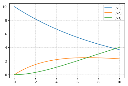
import tellurium as te

# Load an antimony model
ant_model = '''
    S1 -> S2; k1*S1;
    S2 -> S3; k2*S2;

    k1= 0.1; k2 = 0.2;
    S1 = 10; S2 = 0; S3 = 0;
'''
# At the most basic level one can load the SBML model directly using libRoadRunner
print('---  load using roadrunner ---')
import roadrunner
# convert to SBML model
sbml_model = te.antimonyToSBML(ant_model)
r = roadrunner.RoadRunner(sbml_model)
result = r.simulate(0, 10, 100)
r.plot(result)

# The method loada is simply a shortcut to loadAntimonyModel
print('---  load using tellurium ---')
r = te.loada(ant_model)
result = r.simulate (0, 10, 100)
r.plot(result)

# same like
r = te.loadAntimonyModel(ant_model)
--- load using roadrunner ---

--- load using tellurium ---
Interconversion Utilities
Use these routines to interconvert verious standard formats
- tellurium.antimonyToSBML(ant)[source]
Convert Antimony to SBML string.
- Parameters:
ant (str | file) – Antimony string or file
- Returns:
SBML
- Return type:
str
- tellurium.antimonyToCellML(ant)[source]
Convert Antimony to CellML string.
- Parameters:
ant (str | file) – Antimony string or file
- Returns:
CellML
- Return type:
str
- tellurium.sbmlToAntimony(sbml, removeFunctionDefinitions=None)[source]
Convert SBML to antimony string.
- Parameters:
sbml (str | file) – SBML string or file
- Returns:
Antimony
- Return type:
str
- tellurium.sbmlToCellML(sbml)[source]
Convert SBML to CellML string.
- Parameters:
sbml (str | file) – SBML string or file
- Returns:
CellML
- Return type:
str
- tellurium.cellmlToAntimony(cellml)[source]
Convert CellML to antimony string.
- Parameters:
cellml (str | file) – CellML string or file
- Returns:
antimony
- Return type:
str
- tellurium.cellmlToSBML(cellml)[source]
Convert CellML to SBML string.
- Parameters:
cellml (str | file) – CellML string or file
- Returns:
SBML
- Return type:
str
Tellurium can convert between Antimony, SBML, and CellML.
import tellurium as te

# antimony model
ant_model = """
    S1 -> S2; k1*S1;
    S2 -> S3; k2*S2;

    k1= 0.1; k2 = 0.2;
    S1 = 10; S2 = 0; S3 = 0;
"""

# convert to SBML
sbml_model = te.antimonyToSBML(ant_model)
print('sbml_model')
print('*'*80)
# print first 10 lines
for line in list(sbml_model.splitlines())[:10]:
    print(line)
print('...')

# convert to CellML
cellml_model = te.antimonyToCellML(ant_model)
print('cellml_model (from Antimony)')
print('*'*80)
# print first 10 lines
for line in list(cellml_model.splitlines())[:10]:
    print(line)
print('...')

# or from the sbml
cellml_model = te.sbmlToCellML(sbml_model)
print('cellml_model (from SBML)')
print('*'*80)
# print first 10 lines
for line in list(cellml_model.splitlines())[:10]:
    print(line)
print('...')
sbml_model
****************************************************************************
<?xml version="1.0" encoding="UTF-8"?>
<!-- Created by libAntimony version v2.9.4 with libSBML version 5.15.0. -->
<sbml xmlns="http://www.sbml.org/sbml/level3/version1/core" level="3" version="1">
  <model id="__main" name="__main">
    <listOfCompartments>
      <compartment sboTerm="SBO:0000410" id="default_compartment" spatialDimensions="3" size="1" constant="true"/>
    </listOfCompartments>
    <listOfSpecies>
      <species id="S1" compartment="default_compartment" initialConcentration="10" hasOnlySubstanceUnits="false" boundaryCondition="false" constant="false"/>
      <species id="S2" compartment="default_compartment" initialConcentration="0" hasOnlySubstanceUnits="false" boundaryCondition="false" constant="false"/>
...
cellml_model (from Antimony)
****************************************************************************
<?xml version="1.0"?>
<model xmlns:cellml="http://www.cellml.org/cellml/1.1#" xmlns="http://www.cellml.org/cellml/1.1#" name="__main">
<component name="__main">
<variable initial_value="10" name="S1" units="dimensionless"/>
<variable initial_value="0" name="S2" units="dimensionless"/>
<variable initial_value="0.1" name="k1" units="dimensionless"/>
<variable name="_J0" units="dimensionless"/>
<variable initial_value="0" name="S3" units="dimensionless"/>
<variable initial_value="0.2" name="k2" units="dimensionless"/>
<variable name="_J1" units="dimensionless"/>
...
cellml_model (from SBML)
****************************************************************************
<?xml version="1.0"?>
<model xmlns:cellml="http://www.cellml.org/cellml/1.1#" xmlns="http://www.cellml.org/cellml/1.1#" name="__main">
<component name="__main">
<variable initial_value="10" name="S1" units="dimensionless"/>
<variable initial_value="0" name="S2" units="dimensionless"/>
<variable initial_value="0" name="S3" units="dimensionless"/>
<variable initial_value="0.1" name="k1" units="dimensionless"/>
<variable initial_value="0.2" name="k2" units="dimensionless"/>
<variable name="_J0" units="dimensionless"/>
<variable name="_J1" units="dimensionless"/>
...
Export Utilities
Use these routines to convert the current model state into other formats, like Matlab, CellML, Antimony and SBML.
- class tellurium.tellurium.ExtendedRoadRunner(*args, **kwargs)[source]
- exportToAntimony(filePath, current=True)[source]
Save current model as Antimony file.
- Parameters:
current (bool) – export current model state
filePath (str) – file path of Antimony file
- exportToCellML(filePath, current=True)[source]
Save current model as CellML file.
- Parameters:
current (bool) – export current model state
filePath (str) – file path of CellML file
- exportToMatlab(filePath, current=True)[source]
Save current model as Matlab file. To save the original model loaded into roadrunner use current=False.
- Parameters:
self (RoadRunner.roadrunner) – RoadRunner instance
filePath (str) – file path of Matlab file
- exportToSBML(filePath, current=True)[source]
Save current model as SBML file.
- Parameters:
current (bool) – export current model state
filePath (str) – file path of SBML file
- getAntimony(current=False, removeFunctionDefinitions=None)[source]
Antimony string of the original model loaded into roadrunner.
- Parameters:
current (bool) – return current model state
removeFunctionDefinitions – remove function definitions
- Returns:
Antimony
- Return type:
str
- getCellML(current=False)[source]
CellML string of the original model loaded into roadrunner.
- Parameters:
current (bool) – return current model state
- Returns:
CellML string
- Return type:
str
- getCurrentAntimony(removeFunctionDefinitions=None)[source]
Antimony string of the current model state.
See also:
getAntimony():returns: Antimony string :rtype: str
- getCurrentCellML()[source]
CellML string of current model state.
See also:
getCellML():returns: CellML string :rtype: str
- getCurrentMatlab()[source]
Matlab string of current model state.
- Parameters:
current (bool) – return current model state
- Returns:
Matlab string
- Return type:
str
- getMatlab(current=False)[source]
Matlab string of the original model loaded into roadrunner.
See also:
getCurrentMatlab():returns: Matlab string :rtype: str
Given a
RoadRunner
instance, you can get an SBML representation of the current state of the
model using getCurrentSBML. You can also get the initial SBML from
when the model was loaded using getSBML. Finally, exportToSBML
can be used to export the current model state to a file.
import tellurium as te
import tempfile

# load model
r = te.loada('S1 -> S2; k1*S1; k1 = 0.1; S1 = 10')
# file for export
f_sbml = tempfile.NamedTemporaryFile(suffix=".xml")

# export current model state
r.exportToSBML(f_sbml.name)

# to export the initial state when the model was loaded
# set the current argument to False
r.exportToSBML(f_sbml.name, current=False)

# The string representations of the current model are available via
str_sbml = r.getCurrentSBML()

# and of the initial state when the model was loaded via
str_sbml = r.getSBML()
print(str_sbml)
<?xml version="1.0" encoding="UTF-8"?>
<!-- Created by libAntimony version v2.9.4 with libSBML version 5.15.0. -->
<sbml xmlns="http://www.sbml.org/sbml/level3/version1/core" level="3" version="1">
  <model id="__main" name="__main">
    <listOfCompartments>
      <compartment sboTerm="SBO:0000410" id="default_compartment" spatialDimensions="3" size="1" constant="true"/>
    </listOfCompartments>
    <listOfSpecies>
      <species id="S1" compartment="default_compartment" initialConcentration="10" hasOnlySubstanceUnits="false" boundaryCondition="false" constant="false"/>
      <species id="S2" compartment="default_compartment" hasOnlySubstanceUnits="false" boundaryCondition="false" constant="false"/>
    </listOfSpecies>
    <listOfParameters>
      <parameter id="k1" value="0.1" constant="true"/>
    </listOfParameters>
    <listOfReactions>
      <reaction id="_J0" reversible="true" fast="false">
        <listOfReactants>
          <speciesReference species="S1" stoichiometry="1" constant="true"/>
        </listOfReactants>
        <listOfProducts>
          <speciesReference species="S2" stoichiometry="1" constant="true"/>
        </listOfProducts>
        <kineticLaw>
          <math xmlns="http://www.w3.org/1998/Math/MathML">
            <apply>
              <times/>
              <ci> k1 </ci>
              <ci> S1 </ci>
            </apply>
          </math>
        </kineticLaw>
      </reaction>
    </listOfReactions>
  </model>
</sbml>
Similar to the SBML functions above, you can also use the functions
getCurrentAntimony and exportToAntimony to get or export the
current Antimony representation.
import tellurium as te
import tempfile

# load model
r = te.loada('S1 -> S2; k1*S1; k1 = 0.1; S1 = 10')
# file for export
f_antimony = tempfile.NamedTemporaryFile(suffix=".txt")

# export current model state
r.exportToAntimony(f_antimony.name)

# to export the initial state when the model was loaded
# set the current argument to False
r.exportToAntimony(f_antimony.name, current=False)

# The string representations of the current model are available via
str_antimony = r.getCurrentAntimony()

# and of the initial state when the model was loaded via
str_antimony = r.getAntimony()
print(str_antimony)
// Created by libAntimony v2.9.4
// Compartments and Species:
species S1, S2;

// Reactions:
_J0: S1 -> S2; k1*S1;

// Species initializations:
S1 = 10;
S2 = ;

// Variable initializations:
k1 = 0.1;

// Other declarations:
const k1;
Tellurium also has functions for exporting the current model state to CellML. These functionalities rely on using Antimony to perform the conversion.
import tellurium as te
import tempfile

# load model
r = te.loada('S1 -> S2; k1*S1; k1 = 0.1; S1 = 10')
# file for export
f_cellml = tempfile.NamedTemporaryFile(suffix=".cellml")

# export current model state
r.exportToCellML(f_cellml.name)

# to export the initial state when the model was loaded
# set the current argument to False
r.exportToCellML(f_cellml.name, current=False)

# The string representations of the current model are available via
str_cellml = r.getCurrentCellML()

# and of the initial state when the model was loaded via
str_cellml = r.getCellML()
print(str_cellml)
<?xml version="1.0"?>
<model xmlns:cellml="http://www.cellml.org/cellml/1.1#" xmlns="http://www.cellml.org/cellml/1.1#" name="__main">
<component name="__main">
<variable initial_value="10" name="S1" units="dimensionless"/>
<variable name="S2" units="dimensionless"/>
<variable initial_value="0.1" name="k1" units="dimensionless"/>
<variable name="_J0" units="dimensionless"/>
<math xmlns="http://www.w3.org/1998/Math/MathML">
<apply>
<eq/>
<ci>_J0</ci>
<apply>
<times/>
<ci>k1</ci>
<ci>S1</ci>
</apply>
</apply>
</math>
<variable name="time" units="dimensionless"/>
<math xmlns="http://www.w3.org/1998/Math/MathML">
<apply>
<eq/>
<apply>
<diff/>
<bvar>
<ci>time</ci>
</bvar>
<ci>S1</ci>
</apply>
<apply>
<minus/>
<ci>_J0</ci>
</apply>
</apply>
</math>
<math xmlns="http://www.w3.org/1998/Math/MathML">
<apply>
<eq/>
<apply>
<diff/>
<bvar>
<ci>time</ci>
</bvar>
<ci>S2</ci>
</apply>
<ci>_J0</ci>
</apply>
</math>
</component>
<group>
<relationship_ref relationship="encapsulation"/>
<component_ref component="__main"/>
</group>
</model>
To export the current model state to MATLAB, use getCurrentMatlab.
import tellurium as te
import tempfile

# load model
r = te.loada('S1 -> S2; k1*S1; k1 = 0.1; S1 = 10')
# file for export
f_matlab = tempfile.NamedTemporaryFile(suffix=".m")

# export current model state
r.exportToMatlab(f_matlab.name)

# to export the initial state when the model was loaded
# set the current argument to False
r.exportToMatlab(f_matlab.name, current=False)

# The string representations of the current model are available via
str_matlab = r.getCurrentMatlab()

# and of the initial state when the model was loaded via
str_matlab = r.getMatlab()
print(str_matlab)
%  How to use:
%
%  __main takes 3 inputs and returns 3 outputs.
%
%  [t x rInfo] = __main(tspan,solver,options)
%  INPUTS:
%  tspan - the time vector for the simulation. It can contain every time point,
%  or just the start and end (e.g. [0 1 2 3] or [0 100]).
%  solver - the function handle for the odeN solver you wish to use (e.g. @ode23s).
%  options - this is the options structure returned from the MATLAB odeset
%  function used for setting tolerances and other parameters for the solver.
%
%  OUTPUTS:
%  t - the time vector that corresponds with the solution. If tspan only contains
%  the start and end times, t will contain points spaced out by the solver.
%  x - the simulation results.
%  rInfo - a structure containing information about the model. The fields
%  within rInfo are:
%     stoich - the stoichiometry matrix of the model
%     floatingSpecies - a cell array containing floating species name, initial
%     value, and indicator of the units being inconcentration or amount
%     compartments - a cell array containing compartment names and volumes
%     params - a cell array containing parameter names and values
%     boundarySpecies - a cell array containing boundary species name, initial
%     value, and indicator of the units being inconcentration or amount
%     rateRules - a cell array containing the names of variables used in a rate rule
%
%  Sample function call:
%     options = odeset('RelTol',1e-12,'AbsTol',1e-9);
%     [t x rInfo] = __main(linspace(0,100,100),@ode23s,options);
%
function [t x rInfo] = __main(tspan,solver,options)
    % initial conditions
    [x rInfo] = model();

    % initial assignments

    % assignment rules

    % run simulation
    [t x] = feval(solver,@model,tspan,x,options);

    % assignment rules

function [xdot rInfo] = model(time,x)
%  x(1)        S1
%  x(2)        S2

% List of Compartments
vol__default_compartment = 1;               %default_compartment

% Global Parameters
rInfo.g_p1 = 0.1;           % k1

if (nargin == 0)

    % set initial conditions
   xdot(1) = 10*vol__default_compartment;           % S1 = S1 [Concentration]
   xdot(2) = 0*vol__default_compartment;            % S2 = S2 [Concentration]

   % reaction info structure
   rInfo.stoich = [
      -1
      1
   ];

   rInfo.floatingSpecies = {                % Each row: [Species Name, Initial Value, isAmount (1 for amount, 0 for concentration)]
      'S1' , 10, 0
      'S2' , 0, 0
   };

   rInfo.compartments = {           % Each row: [Compartment Name, Value]
      'default_compartment' , 1
   };

   rInfo.params = {         % Each row: [Parameter Name, Value]
      'k1' , 0.1
   };

   rInfo.boundarySpecies = {                % Each row: [Species Name, Initial Value, isAmount (1 for amount, 0 for concentration)]
   };

   rInfo.rateRules = {               % List of variables involved in a rate rule
   };

else

    % calculate rates of change
   R0 = rInfo.g_p1*(x(1));

   xdot = [
      - R0
      + R0
   ];
end;


%listOfSupportedFunctions
function z = pow (x,y)
    z = x^y;


function z = sqr (x)
    z = x*x;


function z = piecewise(varargin)
            numArgs = nargin;
            result = 0;
            foundResult = 0;
            for k=1:2: numArgs-1
                    if varargin{k+1} == 1
                            result = varargin{k};
                            foundResult = 1;
                            break;
                    end
            end
            if foundResult == 0
                    result = varargin{numArgs};
            end
            z = result;


function z = gt(a,b)
   if a > b
      z = 1;
   else
      z = 0;
   end


function z = lt(a,b)
   if a < b
      z = 1;
   else
      z = 0;
   end


function z = geq(a,b)
   if a >= b
      z = 1;
   else
      z = 0;
   end


function z = leq(a,b)
   if a <= b
      z = 1;
   else
      z = 0;
   end


function z = neq(a,b)
   if a ~= b
      z = 1;
   else
      z = 0;
   end


function z = and(varargin)
            result = 1;
            for k=1:nargin
               if varargin{k} ~= 1
                  result = 0;
                  break;
               end
            end
            z = result;


function z = or(varargin)
            result = 0;
            for k=1:nargin
               if varargin{k} ~= 0
                  result = 1;
                  break;
               end
            end
            z = result;


function z = xor(varargin)
            foundZero = 0;
            foundOne = 0;
            for k = 1:nargin
                    if varargin{k} == 0
                       foundZero = 1;
                    else
                       foundOne = 1;
                    end
            end
            if foundZero && foundOne
                    z = 1;
            else
              z = 0;
            end


function z = not(a)
   if a == 1
      z = 0;
   else
      z = 1;
   end


function z = root(a,b)
    z = a^(1/b);
The above examples rely on Antimony as in intermediary between formats.
You can use this functionality directly using e.g.
antimony.getCellMLString. A comprehensive set of functions can be
found in the Antimony API
documentation.
import antimony
antimony.loadAntimonyString('''S1 -> S2; k1*S1; k1 = 0.1; S1 = 10''')
ant_str = antimony.getCellMLString(antimony.getMainModuleName())
print(ant_str)
<?xml version="1.0"?>
<model xmlns:cellml="http://www.cellml.org/cellml/1.1#" xmlns="http://www.cellml.org/cellml/1.1#" name="__main">
<component name="__main">
<variable initial_value="10" name="S1" units="dimensionless"/>
<variable name="S2" units="dimensionless"/>
<variable initial_value="0.1" name="k1" units="dimensionless"/>
<variable name="_J0" units="dimensionless"/>
<math xmlns="http://www.w3.org/1998/Math/MathML">
<apply>
<eq/>
<ci>_J0</ci>
<apply>
<times/>
<ci>k1</ci>
<ci>S1</ci>
</apply>
</apply>
</math>
<variable name="time" units="dimensionless"/>
<math xmlns="http://www.w3.org/1998/Math/MathML">
<apply>
<eq/>
<apply>
<diff/>
<bvar>
<ci>time</ci>
</bvar>
<ci>S1</ci>
</apply>
<apply>
<minus/>
<ci>_J0</ci>
</apply>
</apply>
</math>
<math xmlns="http://www.w3.org/1998/Math/MathML">
<apply>
<eq/>
<apply>
<diff/>
<bvar>
<ci>time</ci>
</bvar>
<ci>S2</ci>
</apply>
<ci>_J0</ci>
</apply>
</math>
</component>
<group>
<relationship_ref relationship="encapsulation"/>
<component_ref component="__main"/>
</group>
</model>
Stochastic Simulation
Use these routines to carry out Gillespie style stochastic simulations.
- class tellurium.tellurium.ExtendedRoadRunner(*args, **kwargs)[source]
- getSeed(integratorName='')
Obtain the current seed for this roadrunner object. warnings.warn(“the integrator option is now ignored for this function. So this function now returns the seed used for the existing model and for the global configuration option”) :param seed: The integrator name to get the seed for. If None, the Config seed is returned.
- gillespie(*args, **kwargs)[source]
Run a Gillespie stochastic simulation.
Sets the integrator to gillespie and performs simulation.
rr = te.loada ('S1 -> S2; k1*S1; k1 = 0.1; S1 = 40')
# Simulate from time zero to 40 time units using variable step sizes (classic Gillespie)
result = rr.gillespie (0, 40)
# Simulate on a grid with 10 points from start 0 to end time 40
rr.reset()
result = rr.gillespie (0, 40, 10)
# Simulate from time zero to 40 time units using variable step sizes with given selection list
# This means that the first column will be time and the second column species S1
rr.reset()
result = rr.gillespie (0, 40, selections=['time', 'S1'])
# Simulate on a grid with 20 points from time zero to 40 time units
# using the given selection list
rr.reset()
result = rr.gillespie (0, 40, 20, ['time', 'S1'])
rr.plot(result)
- Parameters:
seed (int) – seed for gillespie
args – parameters for simulate
kwargs – parameters for simulate
- Returns:
simulation results
- setSeed(seed, resetModel=True)
- Sets the seed for all random number generators: any use of ‘distrib’ in the model, any
simultaneously-firing events, and any use of the ‘gillespie’ integrator. Also sets the global seed in the configuration object, so subsequently-created roadrunner objects will be created with the same seed. Setting the seed to -1 (or any negative integer) tells the random number generators to use a seed based on the system clock (in microcseconds) instead.
warnings.warn(“the integrator option is now ignored for this function. So this function now sets the seed used for the existing model and for the global configuration option”) :param seed: The seed to use for the random number generator. :param resetModel: If True, the model will be reset after setting the seed.
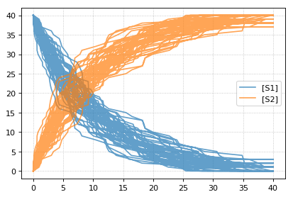
Stochastic simulations can be run by changing the current integrator
type to ‘gillespie’ or by using the r.gillespie function.
import tellurium as te
import numpy as np

r = te.loada('S1 -> S2; k1*S1; k1 = 0.1; S1 = 40')
r.integrator = 'gillespie'
r.integrator.seed = 1234

results = []
for k in range(1, 50):
    r.reset()
    s = r.simulate(0, 40)
    results.append(s)
    r.plot(s, show=False, alpha=0.7)
te.show()
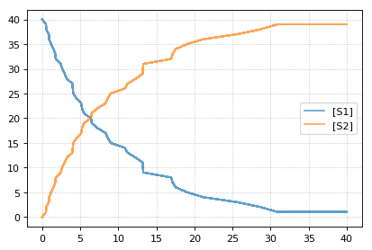
Setting the identical seed for all repeats results in identical traces in each simulation.
results = []
for k in range(1, 20):
    r.reset()
    r.setSeed(123456)
    s = r.simulate(0, 40)
    results.append(s)
    r.plot(s, show=False, loc=None, color='black', alpha=0.7)
te.show()
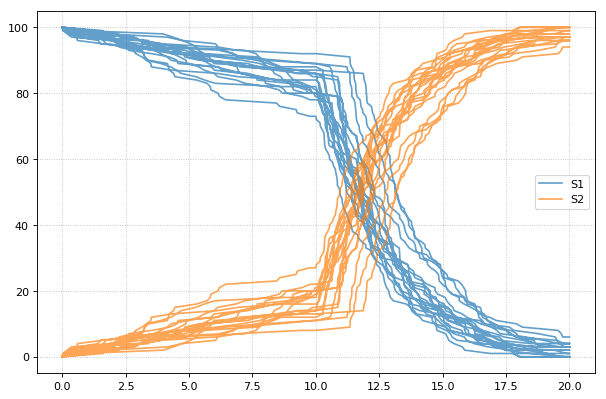
You can combine two timecourse simulations and change e.g. parameter
values in between each simulation. The gillespie method simulates up
to the given end time 10, after which you can make arbitrary changes
to the model, then simulate again.
When using the r.plot function, you can pass the parameter
labels, which controls the names that will be used in the figure
legend, and tag, which ensures that traces with the same tag will
be drawn with the same color (each species within each trace will be
plotted in its own color, but these colors will match trace to trace).
import tellurium as te

r = te.loada('S1 -> S2; k1*S1; k1 = 0.02; S1 = 100')
r.setSeed(1234)
for k in range(1, 20):
    r.resetToOrigin()
    res1 = r.gillespie(0, 10)
    r.plot(res1, show=False) # plot first half of data

    # change in parameter after the first half of the simulation
    # We could have also used an Event in the antimony model,
    # which are described further in the Antimony Reference section
    r.k1 = r.k1*20
    res2 = r.gillespie (10, 20)

    r.plot(res2, show=False) # plot second half of data

te.show()
Math
Use these routines to perform various calculations.
- tellurium.getEigenvalues(m)[source]
Eigenvalues of matrix.
Convenience method for computing the eigenvalues of a matrix m Uses numpy eig to compute the eigenvalues.
- Parameters:
m – numpy array
- Returns:
numpy array containing eigenvalues
- tellurium.rank(A, atol=1e-13, rtol=0)[source]
Estimate the rank (i.e. the dimension of the columnspace) of a matrix.
The algorithm used by this function is based on the singular value decomposition of A.
Parameters
- Andarray
A should be at most 2-D. A 1-D array with length n will be treated as a 2-D with shape (1, n)
- atolfloat
The absolute tolerance for a zero singular value. Singular values smaller than atol are considered to be zero.
- rtolfloat
The relative tolerance. Singular values less than rtol*smax are considered to be zero, where smax is the largest singular value.
If both atol and rtol are positive, the combined tolerance is the maximum of the two; that is:
tol = max(atol, rtol * smax)
Singular values smaller than tol are considered to be zero.
Return value
- rint
The estimated rank of the matrix.
See also
- numpy.linalg.matrix_rank
matrix_rank is basically the same as this function, but it does not provide the option of the absolute tolerance.
- tellurium.nullspace(A, atol=1e-13, rtol=0)[source]
Compute an approximate basis for the nullspace of A.
The algorithm used by this function is based on the singular value decomposition of A.
Parameters
- Andarray
A should be at most 2-D. A 1-D array with length k will be treated as a 2-D with shape (1, k)
- atolfloat
The absolute tolerance for a zero singular value. Singular values smaller than atol are considered to be zero.
- rtolfloat
The relative tolerance. Singular values less than rtol*smax are considered to be zero, where smax is the largest singular value.
If both atol and rtol are positive, the combined tolerance is the maximum of the two; that is:
tol = max(atol, rtol * smax)
Singular values smaller than tol are considered to be zero.
Return value
- nsndarray
If A is an array with shape (m, k), then ns will be an array with shape (k, n), where n is the estimated dimension of the nullspace of A. The columns of ns are a basis for the nullspace; each element in numpy.dot(A, ns) will be approximately zero.
ODE Extraction Methods
Routines to extract ODEs.
- tellurium.getODEsFromSBMLFile(fileName)[source]
Given a SBML file name, this function returns the model as a string of rules and ODEs
>>> te.getODEsFromSBMLFile ('mymodel.xml')
Plotting
Tellurium has a plotting engine which can target either Plotly (when used in a
notebook environment) or Matplotlib. To specify which engine to use, use
te.setDefaultPlottingEngine().
- tellurium.plot(x, y, show=True, **kwargs)[source]
Create a 2D scatter plot.
- Parameters:
x – A numpy array describing the X datapoints. Should have the same number of rows as y.
y – A numpy array describing the Y datapoints. Should have the same number of rows as x.
tag – A tag so that all traces of the same type are plotted using same color/label (for e.g. multiple stochastic traces).
tags – Like tag, but for multiple traces.
name – The name of the trace.
label – The name of the trace.
names – Like name, but for multiple traces to appear in the legend.
labels – The name of the trace.
alpha – Floating point representing the opacity ranging from 0 (transparent) to 1 (opaque).
show – show=True (default) shows the plot, use show=False to plot multiple simulations in one plot
showlegend – Whether to show the legend or not.
mode – Can be set to ‘markers’ to generate scatter plots, or ‘dash’ for dashed lines.
import numpy as np, tellurium as te
result = np.array([[1,2,3,4], [7.2,6.5,8.8,10.5], [9.8, 6.5, 4.3,3.0]])
te.plot(result[:,0], result[:,1], name='Second column', show=False)
te.plot(result[:,0], result[:,2], name='Third column', show=False)
te.show(reset=False) # does not reset the plot after showing plot
te.plot(result[:,0], result[:,3], name='Fourth column', show=False)
te.show()
NOTE: When loading a model with r = te.loada(‘antimony_string’) and calling r.plot(), it is the below tellerium.ExtendedRoadRunner.plot() method below that is called not te.plot().
- tellurium.plotArray(result, loc='upper right', legendOutside=False, show=True, resetColorCycle=True, xlabel=None, ylabel=None, title=None, xlim=None, ylim=None, xscale='linear', yscale='linear', grid=False, labels=None, **kwargs)[source]
Plot an array.
- Parameters:
result – Array to plot, first column of the array must be the x-axis and remaining columns the y-axis
loc (bool) – Location of legend box. Valid strings ‘best’ | upper right’ | ‘upper left’ | ‘lower left’ | ‘lower right’ | ‘right’ | ‘center left’ | ‘center right’ | ‘lower center’ | ‘upper center’ | ‘center’ |
legendOutside= – Set to true if you want the legend outside the axies
color (str) – ‘red’, ‘blue’, etc. to use the same color for every curve
labels – A list of labels for the legend, include as many labels as there are curves to plot
xlabel (str) – x-axis label
ylabel (str) – y-axis label
title (str) – Add plot title
xlim – Limits on x-axis (tuple [start, end])
ylim – Limits on y-axis
xscale – ‘linear’ or ‘log’ scale for x-axis
yscale – ‘linear’ or ‘log’ scale for y-axis
grid (bool) – Show grid
show – show=True (default) shows the plot, use show=False to plot multiple simulations in one plot
resetColorCycle (bool) – If true, resets color cycle on given figure (works with show=False to plot multiple simulations on a single plot)
kwargs – Additional matplotlib keywords like linewidth, linestyle…
If you wish to set the figure size, called plt.figure (figsize=(w,h)) before calling plotArray
import numpy as np, tellurium as te
import matplotlib.pyplot as plt
result = np.array([[1,2,3], [7.2,6.5,8.8], [9.8, 6.5, 4.3]])
plt.figure (figsize=(10,6))
te.plotArray(result, title="My graph", xlim=((1, 5)), labels=["Label 1", "Label 2"],
             yscale='log', linestyle='dashed')
The function tellurium.plotArray assumes that the first column in the array is the x-axis and the second and subsequent columns represent curves on the y-axis.
- class tellurium.tellurium.ExtendedRoadRunner(*args, **kwargs)[source]
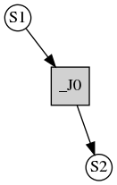
- draw(**kwargs)[source]
Draws an SBMLDiagram of the current model.
To set the width of the output plot provide the ‘width’ argument. Species are drawn as white circles (boundary species shaded in blue), reactions as grey squares. Currently only the drawing of medium-size networks is supported.
- plot(result=None, show=True, xlabel=None, ylabel=None, title=None, linewidth=2, xlim=None, ylim=None, logx=False, logy=False, xscale='linear', yscale='linear', grid=False, ordinates=None, tag=None, labels=None, figsize=(6, 4), savefig=None, dpi=80, alpha=1.0, **kwargs)[source]
Plot roadrunner simulation data.
Plot is called with simulation data to plot as the first argument. If no data is provided the data currently held by roadrunner generated in the last simulation is used. The first column is considered the x axis and all remaining columns the y axis. If the result array has no names, then the current r.selections are used for naming. In this case the dimension of the r.selections has to be the same like the number of columns of the result array.
Curves are plotted in order of selection (columns in result).
In addition to the listed keywords plot supports all matplotlib.pyplot.plot keyword arguments, like color, alpha, linewidth, linestyle, marker, …
sbml = te.getTestModel('feedback.xml')
r = te.loadSBMLModel(sbml)
s = r.simulate(0, 100, 201)
r.plot(s, loc="upper right", linewidth=2.0, lineStyle='-', marker='o', markersize=2.0,
       alpha=0.8, title="Feedback Oscillation", xlabel="time", ylabel="concentration",
       xlim=[0,100], ylim=[-1, 4])
- Parameters:
result – results data to plot (numpy array)
show (bool) – show=True (default) shows the plot, use show=False to plot multiple simulations in one plot
xlabel (str) – x-axis label
ylabel (str) – y-axis label
title (str) – plot title
linewidth (float) – linewidth of the plot
xlim – limits on x-axis (tuple [start, end])
ylim – limits on y-axis
logx (bool) – use log scale for x-axis
logy (bool) – use log scale for y-axis
xscale – ‘linear’ or ‘log’ scale for x-axis
yscale – ‘linear’ or ‘log’ scale for y-axis
grid (bool) – show grid
ordinates – If supplied, only these selections will be plotted (see RoadRunner selections)
tag – If supplied, all traces with the same tag will be plotted with the same color/style
labels – ‘id’ to use species IDs
figsize – If supplied, customize the size of the figure (width,height)
savefig (str) – If supplied, saves the figure to specified location
dpi (int) – Change the dpi of the saved figure
alpha (float) – Change the alpha value of the figure
kwargs – additional matplotlib keywords like marker, lineStyle, …
NOTE: When loading a model with r = te.loada(‘antimony_string’) and calling r.plot(), it is the above tellerium.ExtendedRoadRunner.plot() method below that is called not te.plot().
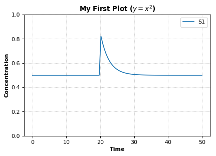
Add plot elements
Example showing how to embelish a graph - change title, axes labels, set axis limit. Example also uses an event to pulse S1.
import tellurium as te, roadrunner

r = te.loada ('''
   $Xo -> S1; k1*Xo;
   S1 -> $X1; k2*S1;

   k1 = 0.2; k2 = 0.4; Xo = 1; S1 = 0.5;
   at (time > 20): S1 = S1 + 0.35
''')

# Simulate the first part up to 20 time units
m = r.simulate (0, 50, 100, ["time", "S1"])
                                                            # using latex syntax to render math
r.plot(m, ylim=(0.,1.), xlabel='Time', ylabel='Concentration', title='My First Plot ($y = x^2$)')
Saving plots
To save a plot, use r.plot and the savefig parameter. Use dpi to specify image quality.
Pass in the save location along with the image name.
import tellurium as te, os
r = te.loada('S1 -> S2; k1*S1; k1 = 0.1; S1 = 10')
result = r.simulate(0, 50, 100)
currentDir = os.getcwd() # gets the current directory
r.plot(title='My plot', xlabel='Time', ylabel='Concentration', dpi=150,
       savefig=currentDir + '\\test.png')  # save image to current directory as "test.png"
The path can be specified as a written out string. The plot can also be saved as a pdf instead of png.
savefig='C:\\Tellurium-Winpython-3.6\\settings\\.spyder-py3\\test.pdf'
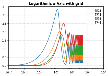
Logarithmic axis
The axis scale can be adapted with the xscale and yscale
settings.
import tellurium as te

r = te.loadTestModel('feedback.xml')
r.integrator.variable_step_size = True
s = r.simulate(0, 50)
r.plot(s, logx=True, xlim=[10E-4, 10E2],
      title="Logarithmic x-Axis with grid", ylabel="concentration");
Plotting multiple simulations
All plotting is done via the r.plot or te.plotArray functions.
To plot multiple curves in one figure use the show=False setting.
import tellurium as te

import numpy as np
import matplotlib.pylab as plt

# Load a model and carry out a simulation generating 100 points
r = te.loada ('S1 -> S2; k1*S1; k1 = 0.1; S1 = 10')
r.draw(width=100)

# get colormap
# Colormap instances are used to convert data values (floats) from the interval [0, 1]
cmap = plt.get_cmap('Blues')

k1_values = np.linspace(start=0.1, stop=1.5, num=15)
max_k1 = max(k1_values)
for k, value in enumerate(k1_values):
    r.reset()
    r.k1 = value
    s = r.simulate(0, 30, 100)

    color = cmap((value+max_k1)/(2*max_k1))
    # use show=False to plot multiple curves in the same figure
    r.plot(s, show=False, title="Parameter variation k1", xlabel="time", ylabel="concentration",
          xlim=[-1, 31], ylim=[-0.1, 11])

te.show()

print('Reference Simulation: k1 = {}'.format(r.k1))
print('Parameter variation: k1 = {}'.format(k1_values))
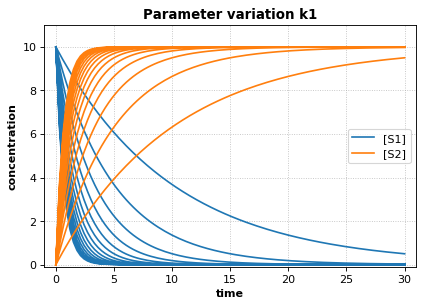
Reference Simulation: k1 = 1.5
Parameter variation: k1 = [0.1 0.2 0.3 0.4 0.5 0.6 0.7 0.8 0.9 1.  1.1 1.2 1.3 1.4 1.5]
Using Tags and Names
Tags can be used to coordinate the color, opacity, and legend names between several sets of data. This can be used to highlight certain features that these datasets have in common. Names allow you to give a more meaningful description of the data in the legend.
import tellurium as te
import numpy as np

for i in range(1, 10):
    x = np.linspace(0, 10, num = 10)
    y = i*x**2 + 10*i

    if i % 2 == 0:
        next_tag = "positive slope"
    else:
        next_tag = "negative slope"
        y = -1*y

    next_name = next_tag + " (i = " + str(i) + ")"
    te.plot(x, y, show = False, tag = next_tag, name = next_name)

te.show()
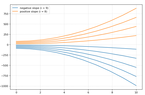
Note that only two items show up in the legend, one for each tag used. In this case, the name found in the legend will match the name of the last set of data plotted using that specific tag. The color and opacity for each tagged groups will also be chosen from the last dataset inputted with that given tag.
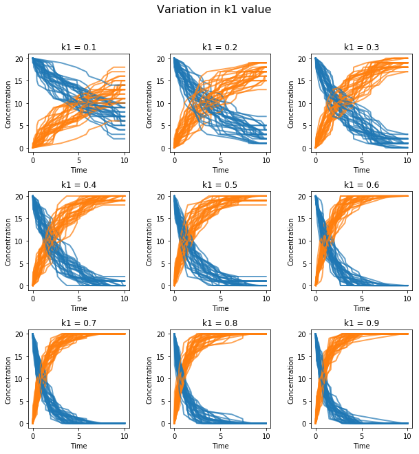
Subplots
te.plotArray can be used in conjunction with matplotlib functions to create subplots.
import tellurium as te
import numpy as np
import matplotlib.pylab as plt

r = te.loada ('S1 -> S2; k1*S1; k1 = 0.1; S1 = 20')
r.setIntegrator('gillespie')
r.integrator.seed = '1234'
kValues = np.linspace(0.1, 0.9, num=9) # generate k1 values

plt.gcf().set_size_inches(10, 10) # size of figure
plt.subplots_adjust(wspace=0.4, hspace=0.4) # adjust the space between subplots
plt.suptitle('Variation in k1 value', fontsize=16) # main title

for i in range(1, len(kValues) + 1):
    r.k1 = kValues[i - 1]
    # designates number of subplots (row, col) and spot to plot next
    plt.subplot(3, 3, i)
    for j in range(1, 30):
        r.reset()
        s = r.simulate(0, 10)
        t = "k1 = " + '{:.1f}'.format(kValues[i - 1])
        # plot each subplot, use show=False to save multiple traces
        te.plotArray(s, show=False, title=t, xlabel='Time',
                     ylabel='Concentration', alpha=0.7)
External Plotting
For those more familiar with plotting in Python, other libraries such as matplotlib.pylab
offer a wider range of plotting options. To use these external libraries, extract the simulation
timecourse data returned from r.simulate. Data is returned in the form of a dictionary/NamedArray,
so specific elements can easily be extracted using the species name as the key.
import tellurium as te
import matplotlib.pylab as plt

antimonyString = ('''
model feedback()
// Reactions:
J0: Nan1 + Mol -> Nan1Mol; (K1*Nan1*Mol);
J1: Nan1Mol -> Nan1 + Mol; (K_1*Nan1Mol);
J2: Nan1Mol + Nan2 -> Nan1MolNan2; (K2*Nan1Mol*Nan2)
J3: Nan1MolNan2 + GeneOff -> GeneOn; (K3*Nan1MolNan2*GeneOff);
J4: GeneOn -> Nan1MolNan2 + GeneOff; (K_3*GeneOn);

// Species initializations:
Nan1 = 0.0001692; Mol = 0.0001692/2; Nan2 = 0.0001692; Nan1Mol = 0;
Nan1MolNan2 = 0; GeneOff = 5*10^-5; GeneOn = 0;

// Variable initialization:
K1 = 6.1*10^5; K_1 = 8*10^-5; K2 = 3.3*10^5; K_2 = 5.7*10^-8;  K3 = 1*10^5; K_3 = 0;
end''')

r = te.loada(antimonyString)
results = r.simulate(0,0.5,1000)
r.plot()

plt.figure(figsize=(30,10));
plt.rc('font', size=30);

plt.subplot(1,2,1);
plt.plot(results['time'], results['[Nan2]'], 'r', results['time'], results['[Nan1MolNan2]'], 'b');
plt.legend({'Nan2', 'Nan1MolNan2'});

plt.subplot(1,2,2);
plt.plot(results['time'], results['[GeneOff]'], 'r', results['time'], results['[GeneOn]'], 'b');
plt.legend({'GeneOff', 'GeneOn'});
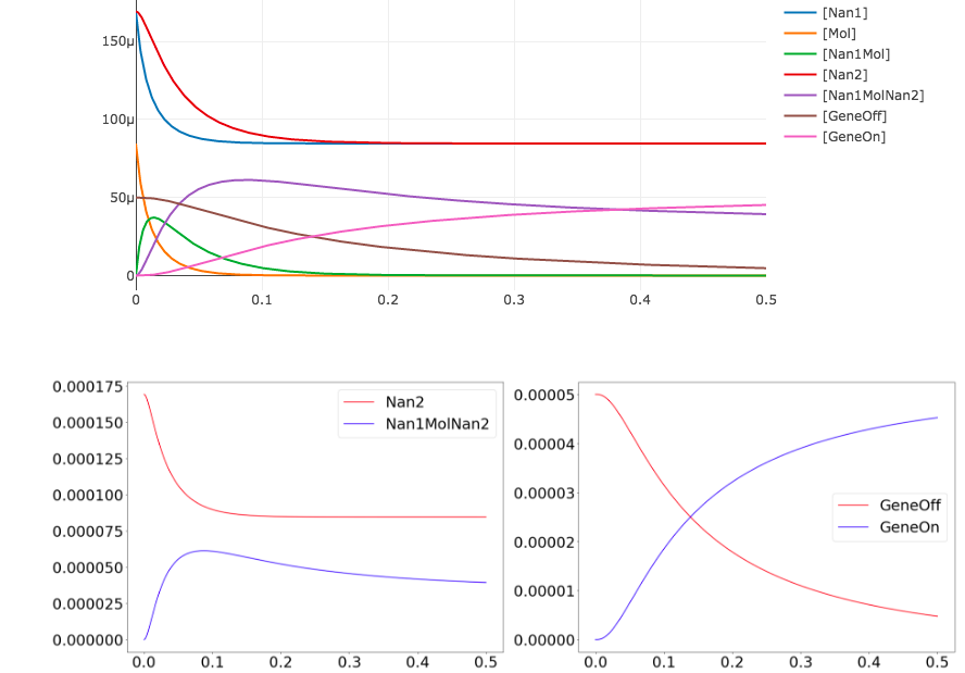
Note that we can extract all the time course data for a specific species such as Nan2 by calling results['[Nan2]'].
The extract brackets [ ] around Nan2 may or may not be required depending on if the units are in terms of
concentration or just a count. To check, simply print out results and you can see the names of each species.
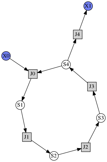
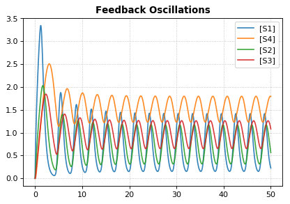
Draw diagram
This example shows how to draw a network diagram, requires graphviz.
import tellurium as te


r = te.loada('''
model feedback()
   // Reactions:http://localhost:8888/notebooks/core/tellurium_export.ipynb#
   J0: $X0 -> S1; (VM1 * (X0 - S1/Keq1))/(1 + X0 + S1 +   S4^h);
   J1: S1 -> S2; (10 * S1 - 2 * S2) / (1 + S1 + S2);
   J2: S2 -> S3; (10 * S2 - 2 * S3) / (1 + S2 + S3);
   J3: S3 -> S4; (10 * S3 - 2 * S4) / (1 + S3 + S4);
   J4: S4 -> $X1; (V4 * S4) / (KS4 + S4);

  // Species initializations:
  S1 = 0; S2 = 0; S3 = 0;
  S4 = 0; X0 = 10; X1 = 0;

  // Variable initialization:
  VM1 = 10; Keq1 = 10; h = 10; V4 = 2.5; KS4 = 0.5;
end''')

# simulate using variable step size
r.integrator.setValue('variable_step_size', True)
s = r.simulate(0, 50)
# draw the diagram
r.draw(width=200)
# and the plot
r.plot(s, title="Feedback Oscillations", ylabel="concentration", alpha=0.9);
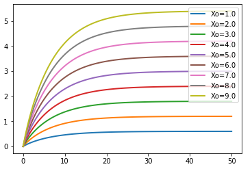
Parameter Scans
To study the consequences of varying a specific parameter value or initial concentration on a simulation,
iteratively adjust the given parameter over a range of values of interest and re-run the simulation.
Using the show parameter and te.show we can plot all these simulations on a single figure.
import tellurium as te
import roadrunner
import numpy as np

r = te.loada("""
     $Xo -> A; k1*Xo;
      A -> B; kf*A - kr*B;
      B -> ; k2*B;

      Xo = 5
      k1 = 0.1; k2 = 0.5;
      kf = 0.3; kr = 0.4
""")

for Xo in np.arange(1.0, 10, 1):
    r.reset()
    r.Xo = Xo
    m = r.simulate (0, 50, 100, ['time', 'A'])
    te.plotArray (m, show=False, labels=['Xo='+str(Xo)], resetColorCycle=False)
te.show()
Parameter Uncertainty Modeling
In most systems, some parameters are more sensitve to perturbations than others. When studying these systems, it is important to understand which parameters are highly sensitive, as errors (i.e. measurement error) introduced to these variables can create drastic differences between experimental and simulated results. To study the sensitivity of these parameters, we can sweep over a range of values as we did in the parameter scan example above. These ranges represent our uncertainty in the value of the parameter, and those parameters that create highly variable results in some measure of an output variable are deemed to be sensitive.
import numpy as np
import tellurium as te
import roadrunner
import antimony
import matplotlib.pyplot as plt
import math

antimonyString = ('''
model feedback()
  // Reactions:
  J0: Nan1 + Mol -> Nan1Mol; (K1*Nan1*Mol);
  J1: Nan1Mol -> Nan1 + Mol; (K_1*Nan1Mol);
  J2: Nan1Mol + Nan2 -> Nan1MolNan2; (K2*Nan1Mol*Nan2)
  J3: Nan1MolNan2 + GeneOff -> GeneOn; (K3*Nan1MolNan2*GeneOff);
  J4: GeneOn -> Nan1MolNan2 + GeneOff; (K_3*GeneOn);

  // Species initializations:
  Nan1 = 0.0001692; Mol = 0.0001692/2; Nan2 = 0.0001692; Nan1Mol = 0;
  Nan1MolNan2 = 0; GeneOff = 5*10^-5; GeneOn = 0;

  // Variable initialization:
  K1 = 6.1*10^5; K_1 = 8*10^-5; K2 = 3.3*10^5; K_2 = 5.7*10^-8;  K3 = 1*10^5; K_3 = 0;
end''')

r = te.loada (model.antimonyString)

def plot_param_uncertainty(model, startVal, name, num_sims):
    stdDev = 0.6

    # assumes initial parameter estimate as mean and iterates 60% above and below.
    vals = np.linspace((1-stdDev)*startVal, (1+stdDev)*startVal, 100)
    for val in vals:
        r.resetToOrigin()
        exec("r.%s = %f" % (name, val))
        result = r.simulate(0,0.5,1000, selections = ['time', 'GeneOn'])
        plt.plot(result[:,0],result[:,1])
        plt.title("uncertainty in " + name)
    plt.legend(["GeneOn"])
    plt.xlabel("Time (hours)")
    plt.ylabel("Concentration")

startVals = r.getGlobalParameterValues();
names = list(enumerate([x for x in r.getGlobalParameterIds() if ("K" in x or "k" in x)]));

n = len(names) + 1;
dim = math.ceil(math.sqrt(n))
for i,next_param in enumerate(names):
    plt.subplot(dim,dim,i+1)
    plot_param_uncertainty(r, startVals[next_param[0]], next_param[1], 100)

plt.tight_layout()
plt.show()

In the above code, the exec command is used to set the model parameters to their given value (i.e. r.K1 = 1.5) and
the code sweeps through all the given parameters of interests (names).
Above, we see that the K3 parameter produces the widest distribution of outcomes, and is thus the most sensitive
under the given model, taking into account its assumptions and approximate parameter values. On the other hand, variations in K_1, K1, and K_3
seem to have very little effect on the outcome of the system.
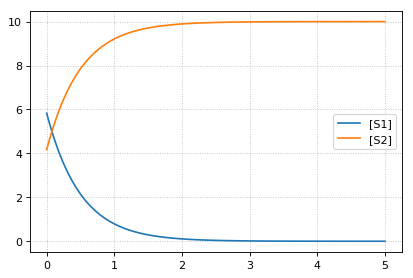
Model Reset
The reset function of a
RoadRunner
instance reset the system variables (usually species concentrations) to
their respective initial values. resetAll resets variables to their CURRENT initial as well as resets parameters.
resetToOrigin completely resets the model.
import tellurium as te
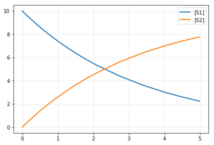
r = te.loada ('S1 -> S2; k1*S1; k1 = 0.1; S1 = 10')
r.integrator.setValue('variable_step_size', True)
# simulate model
sim1 = r.simulate(0, 5)
print('*** sim1 ***')
r.plot(sim1)
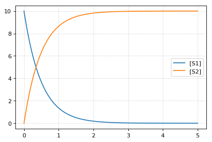
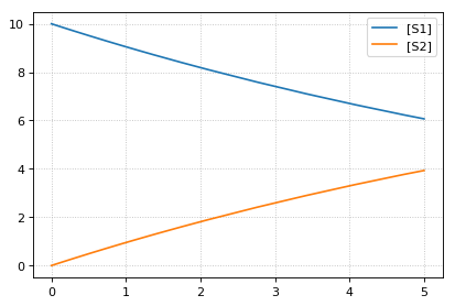
# continue from end concentration of sim1
r.k1 = 2.0
sim2 = r.simulate(0, 5)
print('-- sim2 --')
print('continue simulation from final concentrations with changed parameter')
r.plot(sim2)
# Reset initial concentrations, does not affect the changed parameter
r.reset()
sim3 = r.simulate(0, 5)
print('-- sim3 --')
print('reset initial concentrations but keep changed parameter')
r.plot(sim3)
# Change CURRENT initial of k1, resetAll clears parameter but
# resets to CURRENT initial
r.setValue('init(k1)', 0.3)
r.resetAll()
sim4 = r.simulate(0, 5)
print('-- sim4 --')
print('reset to CURRENT initial of k1, reset to initial parameters')
print('k1 = ' + str(r.k1))
r.plot(sim4)
# Reset model to the state it was loaded
r.resetToOrigin()
sim5 = r.simulate(0, 5)
print('-- sim5 --')
print('reset all to origin')
r.plot(sim5);
* sim1 *

-- sim2 --
continue simulation from final concentrations with changed parameter
-- sim3 --
reset initial concentrations but keep changed parameter
-- sim4 --
reset to CURRENT initial of k1, reset to initial parameters
k1 = 0.3
-- sim5 --
reset all to origin
jarnac Short-cuts
Routines to support the Jarnac compatibility layer
- class tellurium.tellurium.ExtendedRoadRunner(*args, **kwargs)[source]
- bs()[source]
ExecutableModel.getBoundarySpeciesIds()
Returns a vector of boundary species Ids.
- Parameters:
index (numpy.ndarray) – (optional) an index array indicating which items to return.
- Returns:
a list of boundary species ids.
- dv()[source]
RoadRunner::getRatesOfChange()
Returns the rates of change of all floating species. The order of species is given by the order of Ids returned by getFloatingSpeciesIds()
- Returns:
a named array of floating species rates of change.
- Return type:
numpy.ndarray
- fjac()[source]
RoadRunner.getFullJacobian()
Compute the full Jacobian at the current operating point.
This is the Jacobian of ONLY the floating species.
- ps()[source]
ExecutableModel.getGlobalParameterIds([index])
Return a list of global parameter ids.
- Returns:
a list of global parameter ids.
- rs()[source]
ExecutableModel.getReactionIds()
Returns a vector of reaction Ids.
- Parameters:
index (numpy.ndarray) – (optional) an index array indicating which items to return.
- Returns:
a list of reaction ids.
- rv()[source]
ExecutableModel.getReactionRates([index])
Returns a vector of reaction rates (reaction velocity) for the current state of the model. The order of reaction rates is given by the order of Ids returned by getReactionIds()
- Parameters:
index (numpy.ndarray) – (optional) an index array indicating which items to return.
- Returns:
an array of reaction rates.
- Return type:
numpy.ndarray
Stoichiometry
- sm()[source]
RoadRunner.getFullStoichiometryMatrix()
Get the stoichiometry matrix that coresponds to the full model, even it it was converted via conservation conversion.
- sv()[source]
ExecutableModel.getFloatingSpeciesConcentrations([index])
Returns a vector of floating species concentrations. The order of species is given by the order of Ids returned by getFloatingSpeciesIds()
- Parameters:
index (numpy.ndarray) – (optional) an index array indicating which items to return.
- Returns:
an array of floating species concentrations.
- Return type:
numpy.ndarray
Test Models
RoadRunner has built into it a number of predefined models that can be use to easily try and test tellurium.
- tellurium.loadTestModel(string)[source]
Loads particular test model into roadrunner.
rr = te.loadTestModel('feedback.xml')
- Returns:
RoadRunner instance with test model loaded
- tellurium.getTestModel(string)[source]
SBML of given test model as a string.
# load test model as SBML
sbml = te.getTestModel('feedback.xml')
r = te.loadSBMLModel(sbml)
# simulate
r.simulate(0, 100, 20)
- Returns:
SBML string of test model
- tellurium.listTestModels()[source]
List roadrunner SBML test models.
print(te.listTestModels())
- Returns:
list of test model paths
Test models
import tellurium as te

# To get the builtin models use listTestModels
print(te.listTestModels())
['EcoliCore.xml', 'linearPathwayClosed.xml', 'test_1.xml', 'linearPathwayOpen.xml', 'feedback.xml']
Load test model
# To load one of the test models use loadTestModel:
# r = te.loadTestModel('feedback.xml')
# result = r.simulate (0, 10, 100)
# r.plot (result)

# If you need to obtain the SBML for the test model, use getTestModel
sbml = te.getTestModel('feedback.xml')

# To look at one of the test model in Antimony form:
ant = te.sbmlToAntimony(te.getTestModel('feedback.xml'))
print(ant)
// Created by libAntimony v2.9.4
model *feedback()

  // Compartments and Species:
  compartment compartment_;
  species S1 in compartment_, S2 in compartment_, S3 in compartment_, S4 in compartment_;
  species $X0 in compartment_, $X1 in compartment_;

  // Reactions:
  J0: $X0 => S1; J0_VM1*(X0 - S1/J0_Keq1)/(1 + X0 + S1 + S4^J0_h);
  J1: S1 => S2; (10*S1 - 2*S2)/(1 + S1 + S2);
  J2: S2 => S3; (10*S2 - 2*S3)/(1 + S2 + S3);
  J3: S3 => S4; (10*S3 - 2*S4)/(1 + S3 + S4);
  J4: S4 => $X1; J4_V4*S4/(J4_KS4 + S4);

  // Species initializations:
  S1 = 0;
  S2 = 0;
  S3 = 0;
  S4 = 0;
  X0 = 10;
  X1 = 0;

  // Compartment initializations:
  compartment_ = 1;

  // Variable initializations:
  J0_VM1 = 10;
  J0_Keq1 = 10;
  J0_h = 10;
  J4_V4 = 2.5;
  J4_KS4 = 0.5;

  // Other declarations:
  const compartment_, J0_VM1, J0_Keq1, J0_h, J4_V4, J4_KS4;
end
Running external tools
Routines to run external tools.
- tellurium.runTool(toolFileName)[source]
Call an external application called toolFileName. Note that .exe extension may be omitted for windows applications.
Include any arguments in arguments parameter.
Example: returnString = te.runTool ([‘myplugin’, ‘arg1’, ‘arg2’])
If the external tool writes to stdout, this will be captured and returned.
- Parameters:
toolFileName – argument to external tool
- Returns:
String return by external tool, if any.
Model Methods
Routines flattened from model, saves typing and easier for finding the methods
- class tellurium.tellurium.ExtendedRoadRunner(*args, **kwargs)[source]
- getBoundarySpeciesConcentrations([index])
Returns a vector of boundary species concentrations. The order of species is given by the order of Ids returned by getBoundarySpeciesIds()
- Parameters:
index (numpy.ndarray) – (optional) an index array indicating which items to return.
- Returns:
an array of the boundary species concentrations.
- Return type:
numpy.ndarray.
given by the order of Ids returned by getBoundarySpeciesIds()
- Parameters:
index (numpy.ndarray) – (optional) an index array indicating which items to return.
- Returns:
an array of the boundary species concentrations.
- Return type:
numpy.ndarray.
- getBoundarySpeciesIds()
Returns a vector of boundary species Ids.
- Parameters:
index (numpy.ndarray) – (optional) an index array indicating which items to return.
- Returns:
a list of boundary species ids.
- getCompartmentIds([index])
Returns a vector of compartment identifier symbols.
- Parameters:
index (None or numpy.ndarray) – A array of compartment indices indicating which compartment ids to return.
- Returns:
a list of compartment ids.
- getCompartmentVolumes([index])
Returns a vector of compartment volumes. The order of volumes is given by the order of Ids returned by getCompartmentIds()
- Parameters:
index (numpy.ndarray) – (optional) an index array indicating which items to return.
- Returns:
an array of compartment volumes.
- Return type:
numpy.ndarray.
- getConservedMoietyValues([index])
Returns a vector of conserved moiety volumes. The order of values is given by the order of Ids returned by getConservedMoietyIds()
- Parameters:
index (numpy.ndarray) – (optional) an index array indicating which items to return.
- Returns:
an array of conserved moiety values.
- Return type:
numpy.ndarray.
- getFloatingSpeciesConcentrations([index])
Returns a vector of floating species concentrations. The order of species is given by the order of Ids returned by getFloatingSpeciesIds()
- Parameters:
index (numpy.ndarray) – (optional) an index array indicating which items to return.
- Returns:
an array of floating species concentrations.
- Return type:
numpy.ndarray
- getFloatingSpeciesIds()
Return a list of floating species sbml ids.
- getGlobalParameterIds([index])
Return a list of global parameter ids.
- Returns:
a list of global parameter ids.
- getGlobalParameterValues([index])
Return a vector of global parameter values. The order of species is given by the order of Ids returned by getGlobalParameterIds()
- Parameters:
index (numpy.ndarray) – (optional) an index array indicating which items to return.
- Returns:
an array of global parameter values.
- Return type:
numpy.ndarray.
- getNumBoundarySpecies()
Returns the number of boundary species in the model.
- getNumCompartments()
Returns the number of compartments in the model.
- Return type:
int
- getNumConservedMoieties()
Returns the number of conserved moieties in the model.
- Return type:
int
- getNumFloatingSpecies()
Returns the number of floating species in the model.
- getNumGlobalParameters()
Returns the number of global parameters in the model.
- getNumReactions()
Returns the number of reactions in the model.
- getRatesOfChange()
Returns the rates of change of all floating species. The order of species is given by the order of Ids returned by getFloatingSpeciesIds()
- Returns:
a named array of floating species rates of change.
- Return type:
numpy.ndarray
- getReactionIds()
Returns a vector of reaction Ids.
- Parameters:
index (numpy.ndarray) – (optional) an index array indicating which items to return.
- Returns:
a list of reaction ids.
- getReactionRates([index])
Returns a vector of reaction rates (reaction velocity) for the current state of the model. The order of reaction rates is given by the order of Ids returned by getReactionIds()
- Parameters:
index (numpy.ndarray) – (optional) an index array indicating which items to return.
- Returns:
an array of reaction rates.
- Return type:
numpy.ndarray
Stoichiometry