Quick Start

To get started using Tellurium, either install Tellurium in your favorite Python environment with

pip install tellurium

or install the latest Tellurium/Spyder front end. For more details, see the Tellurium README.

Then, follow the examples below to get an idea of how to load and simulate models.

Simple Example

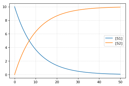
This shows how to set up a simple model in Tellurium and solve it as an ODE. Tellurium uses a human-readable representation of SBML models called Antimony. The Antimony code for this example contains a single reaction with associated kinetics. After creating the Antimony string, use the loada function to load it into the RoadRunner simulator. A RoadRunner instance has a method simulate that can be used to run timecourse simulations of a model, as shown below.

import tellurium as te
r = te.loada('S1 -> S2; k1*S1; k1 = 0.1; S1 = 10')
r.simulate(0, 50, 100)
r.plot()

More Complex Example

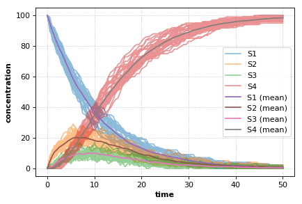
Tellurium can also handle stochastic models. This example shows how to select Tellurium’s stochastic solver. The underlying simulation engine used by Tellurium implements a Gibson direct method for simulating this model.

import tellurium as te
import numpy as np

r = te.loada('''
    J1: S1 -> S2;  k1*S1;
    J2: S2 -> S3; k2*S2 - k3*S3
    # J2_1: S2 -> S3; k2*S2
    # J2_2: S3 -> S2; k3*S3;
    J3: S3 -> S4; k4*S3;

    k1 = 0.1; k2 = 0.5; k3 = 0.5; k4 = 0.5;
    S1 = 100;
''')

# use a stochastic solver
r.integrator = 'gillespie'
r.integrator.seed = 1234
# selections specifies the output variables in a simulation
selections = ['time'] + r.getBoundarySpeciesIds() + r.getFloatingSpeciesIds()
r.integrator.variable_step_size = False

# run repeated simulation
Ncol = len(r.selections)
Nsim = 30
points = 101
s_sum = np.zeros(shape=[points, Ncol])
for k in range(Nsim):
    r.resetToOrigin()
    s = r.simulate(0, 50, points, selections=selections)
    s_sum += s
    # use show=False to add traces to the current plot
    # instead of starting a new one, equivalent to MATLAB hold on
    r.plot(s, alpha=0.5, show=False)

# add mean curve, legend, show everything and set labels, titels, ...
fig = te.plot(s[:,0], s_sum[:,1:]/Nsim, names=[x + ' (mean)' for x in selections[1:]], title="Stochastic simulation", xlabel="time", ylabel="concentration")