Parameter Scan
ParameterScan is a package for Tellurium that provides a different way to run simulations and plot graphs than given in the standard Tellurium library. While the standard syntax in Tellurium asks you to put parameters, such as the amount of time for the simulation to run, as arguments in the simulation function, ParameterScan allows you to set these values before calling the function. This is especially useful for more complicated 3D plots that often take many arguments to customize. Therefore, ParameterScan also provides several plotting options that would be cumbersome to handle using the traditional approach. This tutorial will go over how to use all of ParameterScan’s functionality.
Loading a Model
To use ParameterScan you will need to import it. The easiest way to do this is the command ‘from tellurium import ParameterScan’ after the standard ‘import tellurium as te’.
import tellurium as te
from tellurium import ParameterScan

cell = '''
    $Xo -> S1; vo;
    S1 -> S2; k1*S1 - k2*S2;
    S2 -> $X1; k3*S2;

    vo = 1
    k1 = 2; k2 = 0; k3 = 3;
'''

rr = te.loadAntimonyModel(cell)
p = ParameterScan(rr)

p.startTime = 0
p.endTime = 20
p.numberOfPoints = 50
p.width = 2
p.xlabel = 'Time'
p.ylabel = 'Concentration'
p.title = 'Cell'

p.plotArray()
After you load the model, you can use it to create an object of ParameterScan. This allows you to set many different parameters and easily change them.
Class Methods
These are the methods of the ParameterScan class.
plotArray()
The plotArray() method works much the same as te.plotArray(), but with some increased functionality. It automatically runs a simulation based on the given parameters, and plots a graph of the results. Accepted parameters are startTime, endTime, numberOfPoints, width, color, xlabel, ylabel, title, integrator, and selection.
plotGraduatedArray()
This method runs several simulations, each one with a slightly higher starting concentration of a chosen species than the last. It then plots the results. Accepted parameters are startTime, endTime, value, startValue, endValue, numberOfPoints, width, color, xlabel, ylabel, title, integrator, and polyNumber.
plotPolyArray()
This method runs the same simulation as plotGraduatedArray(), but plots each graph as a polygon in 3D space. Accepted parameters are startTime, endTime, value, startValue, endValue, numberOfPoints, color, alpha, xlabel, ylabel, title, integrator, and polyNumber.
plotMultiArray(param1, param1Range, param2, param2Range)
This method plots a grid of arrays with different starting conditions. It is the only method in ParameterScan that takes arguments when it is called. The two param arguments specify the species or constant that should be set, and the range arguments give the different values that should be simulated with. The resulting grid is an array for each possible combination of the two ranges. For instance, plotMultiArray(‘k1’, [1, 2], ‘k2’, [1, 2, 3]) would result in a grid of six arrays, one with k1 = 1 and k2 = 1, the next with k1 = 1 and k2 = 2, and so on. The advantage of this method is that you can plot multiple species in each array. Accepted parameters are startTime, endTime, numberOfPoints, width, title, and integrator.
plotSurface()
This method produces a color-coded 3D surface based on the concentration of one species and the variation of two factors (usually time and an equilibrium constant). Accepted parameters are startTime, endTime, numberOfPoints, startValue, endValue, independent, dependent, color, xlabel, ylabel, title, integrator, colormap, colorbar, and antialias.
plot2DParameterScan(p1, p1Range, p2, p2Range)
Create a 2D parameter scan and plots the results. The two parameters p1, p2 are the id of the first and second parameter. p1Range and p2Range are the range of the first and second parameter respectively. Parameters start and end represents the starting time and ending time, and points is the number of points to simulate. Will generate a 2D plot containing multiple graphs of the given parameters at various values in the given ranges.
createColormap(color1, color2)
This method allows you to create a custom colormap for plotSurface(). It returns a colormap that stretches between color1 and color2. Colors can be input as RGB tuplet lists (i.e. [0.5, 0, 1]), or as strings with either a standard color name or a hex value. The first color becomes bottom of the colormap (i.e. lowest values in plotArray()) and the second becomes the top.
createColorPoints()
This method creates a color list (i.e. sets ‘color’) spanning the range of a colormap. The colormap can either be predefined or user-defined with createColorMap(). This set of colors will then be applied to arrays, including plotArray(), plotPolyArray(), and plotGraduatedArray(). Note: This method gets the number of colors to generate from the polyNumber parameter. If using it with plotArray() or plotGraduatedArray(), setting this parameter to the number of graphs you are expecting will obtain better results.
Example
Let’s say that we want to examine how the value of a rate constant (parameter) affects how the concentration of a species changes over time. There are several ways this can be done, but the simplest is to use plotGraduatedArray. Here is an example script:
import tellurium as te
from tellurium import ParameterScan

r = te.loada('''
    $Xo -> S1; vo;
    S1 -> S2; k1*S1 - k2*S2;
    S2 -> $X1; k3*S2;

    vo = 1
    k1 = 2; k2 = 0; k3 = 3;
''')

p = ParameterScan(r)

p.endTime = 6
p.numberOfPoints = 100
p.polyNumber = 5
p.startValue = 1
p.endValue = 5
p.value = 'k1'
p.selection = ['S1']

p.plotGraduatedArray()
Another way is to use createColormap() and plotSurface() to create a 3D graph of the same model as above. After loading the model, we can use this code:
p.endTime = 6
p.colormap = p.createColormap([.12,.56,1], [.86,.08,.23])
p.dependent = 'S1'
p.independent = ['time', 'k1']
p.startValue = 1
p.endValue = 5
p.numberOfPoints = 100

p.plotSurface()
Perform Parameter Scan
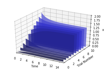
plotPolyArray() example
import tellurium as te

r = te.loada('''
    J1: $Xo -> x; 0.1 + k1*x^4/(k2+x^4);
    x -> $w; k3*x;

    k1 = 0.9;
    k2 = 0.3;
    k3 = 0.7;
    x = 0;
''')

# parameter scan
p = te.ParameterScan(r,
    # settings
    startTime = 0,
    endTime = 15,
    numberOfPoints = 50,
    polyNumber = 10,
    endValue = 1.8,
    alpha = 0.8,
    value = "x",
    selection = "x",
    color = ['#0F0F3D', '#141452', '#1A1A66', '#1F1F7A', '#24248F', '#2929A3',
               '#2E2EB8', '#3333CC', '#4747D1', '#5C5CD6']
)
# plot
p.plotPolyArray()
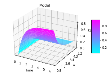
plotSurface() example
r = te.loada('''
    $Xo -> S1; vo;
    S1 -> S2; k1*S1 - k2*S2;
    S2 -> $X1; k3*S2;

    vo = 1
    k1 = 2; k2 = 0; k3 = 3;
''')

# parameter scan
p = te.ParameterScan(r,
    # settings
    startTime = 0,
    endTime = 6,
    numberOfPoints = 50,
    startValue = 1,
    endValue = 5,
    colormap = "cool",
    independent = ["Time", "k1"],
    dependent = "S1",
    xlabel = "Time",
    ylabel = "x",
    title = "Model"
)
# plot
p.plotSurface()
import warnings
warnings.filterwarnings("ignore")
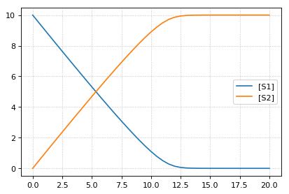
import tellurium as te
from tellurium.analysis.parameterscan import plot2DParameterScan
# model definitions
r = te.loada("""
model test
J0: S1 -> S2; Vmax * (S1/(Km+S1))
S1 = 10; S2 = 0;
Vmax = 1; Km = 0.5;
end
""")
s = r.simulate(0, 20, 41)
r.plot(s)
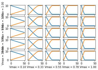
import numpy as np
plot2DParameterScan(r,
p1='Vmax', p1Range=np.linspace(1, 10, num=5),
p2='Vmax', p2Range=np.linspace(0.1, 1.0, num=5),
start=0, end=50, points=101)
Properties
These are the properties of the ParameterScan class.
alpha: Sets opaqueness of polygons in plotPolyArray(). Should be a number from 0-1. Set to 0.7 by default.
color: Sets color for use in all plotting functions except plotSurface() and plotMultiArray(). Should be a list of at least one string. All legal HTML color names are accepted. Additionally, for plotArray() and plotGraduatedArray(), this parameter can determine the appearance of the line as according to PyPlot definitions. For example, setting color to [‘ro’] would produce a graph of red circles. For examples on types of lines in PyPlot, go to http://matplotlib.org/api/pyplot_api.html#matplotlib.pyplot.plot. If there are more graphs than provided color selections, subsequent graphs will start back from the beginning of the list.
colorbar: True shows a color legend for plotSurface(), False does not. Set to True by default.
colormap: The name of the colormap you want to use for plotSurface(). Legal names can be found at http://matplotlib.org/examples/color/colormaps_reference.html and should be strings. Alternatively, you can create a custom colormap using the createColorMap method.
dependent: The dependent variable for plotSurface(). Should be a string of a valid species.
endTime: When the simulation ends. Default is 20.
endValue: For plotGraduatedArray(), assigns the final value of the independent variable other than time. For plotPolyArray() and plotSurface() assigns the final value of the parameter being varied. Should be a string of a valid parameter.
independent: The independent variable for plotSurface(). Should be a list of two strings: one for time, and one for a parameter.
integrator: The integrator used to calculate results for all plotting methods. Set to ‘cvode’ by default, but another option is ‘gillespie.’
legend: A bool that determines whether a legend is displayed for plotArray(), plotGraduatedArray(), and plotMultiArray(). Default is True.
numberOfPoints: Number of points in simulation results. Default is 50. Should be an integer.
polyNumber: The number of graphs for plotGraduatedArray() and plotPolyArray(). Default is 10.
rr: A pointer to a loaded RoadRunner model. ParameterScan() takes it as its only argument.
selection: The species to be shown in the graph in plotArray() and plotMultiArray(). Should be a list of at least one string.
sameColor: Set this to True to force plotGraduatedArray() to be all in one color. Default color is blue, but another color can be chosen via the “color” parameter. Set to False by default.
startTime: When the simulation begins. Default is 0.
startValue: For plotGraduatedArray(), assigns the beginning value of the independent variable other than time. For plotPolyArray() and plotSurface() assigns the beginning value of the parameter being varied. Default is whatever the value is in the loaded model, or if not specified there, 0.
title: Default is no title. If set to a string, it will display above any of the plotting methods.
value: The item to be varied between graphs in plotGraduatedArray() and plotPolyArray(). Should be a string of a valid species or parameter.
width: Sets line width in plotArray(), plotGraduatedArray(), and plotMultiArray(). Won’t have any effect on special line types (see color). Default is 2.5.
xlabel: Sets a title for the x-axis. Should be a string. Not setting it results in an appropriate default; to create a graph with no title for the x-axis, set it to None.
ylabel: Sets a title for the y-axis. Should be a string. Not setting it results in an appropriate default; to create a graph with no title for the x-axis, set it to None.
zlabel: Sets a title for the z-axis. Should be a string. Not setting it results in an appropriate default; to create a graph with no title for the x-axis, set it to None.
SteadyStateScan
This class is part of ParameterScan but provides some added functionality. It allows the user to plot graphs of the steady state values of one or more species as dependent on the changing value of an equilibrium constant on the x-axis. To use it, use the same import statement as before: ‘from tellurium import SteadyStateScan. Then, you can use SteadyStateScan on a loaded model by using ‘ss = SteadyStateScan(rr)’. Right now, the only working method is plotArray(), which needs the parameters of value, startValue, endValue, numberOfPoints, and selection. The parameter ‘value’ refers to the equilibrium constant, and should be the string of the chosen constant. The start and end value parameters are numbers that determine the domain of the x-axis. The ‘numberOfPoints’ parameter refers to the number of data points (i.e. a larger value gives a smoother graph) and ‘selection’ is a list of strings of one or more species that you would like in the graph.
Steady state scan
Using te.ParameterScan.SteadyStateScan for scanning the steady
state.
import tellurium as te
import matplotlib.pyplot as plt
import tellurium as te
import numpy as np
from roadrunner import Config

r = te.loada('''
    $Xo -> S1; vo;
    S1 -> S2; k1*S1 - k2*S2;
    S2 -> $X1; k3*S2;

    vo = 1
    k1 = 2; k2 = 0; k3 = 3;
''')

p = te.SteadyStateScan(r,
    value = 'k3',
    startValue = 2,
    endValue = 3,
    numberOfPoints = 20,
    selection = ['S1', 'S2']
)
p.plotArray()
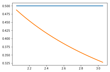
array([[2.05263158, 0.5       , 0.48717949],
       [2.10526316, 0.5       , 0.475     ],
       [2.15789474, 0.5       , 0.46341463],
       [2.21052632, 0.5       , 0.45238095],
       [2.26315789, 0.5       , 0.44186047],
       [2.31578947, 0.5       , 0.43181818],
       [2.36842105, 0.5       , 0.42222222],
       [2.42105263, 0.5       , 0.41304348],
       [2.47368421, 0.5       , 0.40425532],
       [2.52631579, 0.5       , 0.39583333],
       [2.57894737, 0.5       , 0.3877551 ],
       [2.63157895, 0.5       , 0.38      ],
       [2.68421053, 0.5       , 0.37254902],
       [2.73684211, 0.5       , 0.36538462],
       [2.78947368, 0.5       , 0.35849057],
       [2.84210526, 0.5       , 0.35185185],
       [2.89473684, 0.5       , 0.34545455],
       [2.94736842, 0.5       , 0.33928571],
       [3.        , 0.5       , 0.33333333],
       [3.05263158, 0.5       , 0.32758621]])