Usage Examples

All tellurium examples are available as interactive Tellurium or Jupyter notebooks.

To run the examples, clone the git repository:

git clone https://github.com/sys-bio/tellurium.git

and use the Tellurium notebook viewer or Jupyter to open any notebook in the tellurium/examples/notebooks/core directory.

Tellurium Spyder comes with these examples under Tellurium Spyder installation directory. Look for folder called tellurium-winpython-examples.

Basics

Model Loading

To load models use any the following functions. Each function takes a model with the corresponding format and converts it to a RoadRunner simulator instance.

• te.loadAntimonyModel (te.loada): Load an Antimony model.

• te.loadSBMLModel (te.loads): Load an SBML model.

import tellurium as te
te.setDefaultPlottingEngine('matplotlib')

model = """
model test
    compartment C1;
    C1 = 1.0;
    species S1, S2;

    S1 = 10.0;
    S2 = 0.0;
    S1 in C1; S2 in C1;
    J1: S1 -> S2; k1*S1;

    k1 = 1.0;
end
"""
# load models
r = te.loada(model)

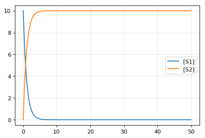
Running Simulations

Simulating a model in roadrunner is as simple as calling the simulate function on the RoadRunner instance r. The simulate acceps three positional arguments: start time, end time, and number of points. The simulate function also accepts the keyword arguments selections, which is a list of variables to include in the output, and steps, which is the number of integration time steps and can be specified instead of number of points.

# simulate from 0 to 50 with 100 steps
r.simulate(0, 50, 100)
# plot the simulation
r.plot()

Integrator and Integrator Settings

To set the integrator use r.setIntegrator(<integrator-name>) or r.integrator = <integrator-name>. RoadRunner supports 'cvode', 'gillespie', and 'rk4' for the integrator name. CVODE uses adaptive stepping internally, regardless of whether the output is gridded or not. The size of these internal steps is controlled by the tolerances, both absolute and relative.

To set integrator settings use r.integrator.<setting-name> = <value> or r.integrator.setValue(<setting-name>, <value>). Here are some important settings for the cvode integrator:

• variable_step_size: Adaptive step-size integration (True/False).

• stiff: Stiff solver for CVODE only (True/False). Enabled by default.

• absolute_tolerance: Absolute numerical tolerance for integrator internal stepping.

• relative_tolerance: Relative numerical tolerance for integrator internal stepping.

Settings for the gillespie integrator:

• seed: The RNG seed for the Gillespie method. You can set this before running a simulation, or leave it alone for a different seed each time. Simulations initialized with the same seed will have the same results.

# what is the current integrator?
print('The current integrator is:')
print(r.integrator)

# enable variable stepping
r.integrator.variable_step_size = True
# adjust the tolerances (can set directly or via setValue)
r.integrator.absolute_tolerance = 1e-3 # set directly via property
r.integrator.setValue('relative_tolerance', 1e-1) # set via a call to setValue

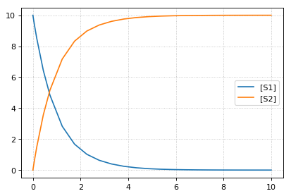
# run a simulation, stop after reaching or passing time 10
r.reset()
results = r.simulate(0, 10)
r.plot()

# print the time values from the simulation
print('Time values:')
print(results[:,0])

The current integrator is:
< roadrunner.Integrator() >
  name: cvode
  settings:
      relative_tolerance: 0.000001
      absolute_tolerance: 0.000000000001
                   stiff: true
       maximum_bdf_order: 5
     maximum_adams_order: 12
       maximum_num_steps: 20000
       maximum_time_step: 0
       minimum_time_step: 0
       initial_time_step: 0
          multiple_steps: false
      variable_step_size: false

Time values:
[0.00000000e+00 3.43225906e-07 3.43260229e-03 3.77551929e-02
 7.20777836e-02 1.60810095e-01 4.37546265e-01 7.14282434e-01
 1.23145372e+00 1.74862501e+00 2.26579629e+00 2.78296758e+00
 3.30013887e+00 3.81731015e+00 4.33448144e+00 4.85165273e+00
 5.36882401e+00 5.88599530e+00 6.40316659e+00 6.92033787e+00
 7.43750916e+00 7.95468045e+00 8.47185173e+00 9.25832855e+00
 1.00000000e+01]

# set integrator to Gillespie solver
r.setIntegrator('gillespie')
# identical ways to set integrator
r.setIntegrator('rk4')
r.integrator = 'rk4'
# set back to cvode (the default)
r.setIntegrator('cvode')

# set integrator settings
r.integrator.setValue('variable_step_size', False)
r.integrator.setValue('stiff', True)

# print integrator settings
print(r.integrator)

< roadrunner.Integrator() >
  name: cvode
  settings:
      relative_tolerance: 0.1
      absolute_tolerance: 0.001
                   stiff: true
       maximum_bdf_order: 5
     maximum_adams_order: 12
       maximum_num_steps: 20000
       maximum_time_step: 0
       minimum_time_step: 0
       initial_time_step: 0
          multiple_steps: false
      variable_step_size: false

Simulation options

The RoadRunner.simulate method is responsible for running simulations using the current integrator. It accepts the following arguments:

• start: Start time.

• end: End time.

• points: Number of points in solution (exclusive with steps, do not pass both). If the output is gridded, the points will be evenly spaced in time. If not, the simulation will stop when it reaches the end time or the number of points, whichever happens first.

• steps: Number of steps in solution (exclusive with points, do not pass both).

# simulate from 0 to 6 with 6 points in the result
r.reset()
# pass args explicitly via keywords
res1 = r.simulate(start=0, end=10, points=6)
print(res1)
r.reset()
# use positional args to pass start, end, num. points
res2 = r.simulate(0, 10, 6)
print(res2)

   time,       [S1],    [S2]
[[    0,         10,       0],
 [    2,    1.23775, 8.76225],
 [    4,   0.253289, 9.74671],
 [    6,  0.0444091, 9.95559],
 [    8, 0.00950381,  9.9905],
 [   10, 0.00207671, 9.99792]]

   time,       [S1],    [S2]
[[    0,         10,       0],
 [    2,    1.23775, 8.76225],
 [    4,   0.253289, 9.74671],
 [    6,  0.0444091, 9.95559],
 [    8, 0.00950381,  9.9905],
 [   10, 0.00207671, 9.99792]]

Selections

The selections list can be used to set which state variables will appear in the output array. By default, it includes all SBML species and the time variable. Selections can be given as an argument to r.simulate.

print('Floating species in model:')
print(r.getFloatingSpeciesIds())
# provide selections to simulate
print(r.simulate(0,10,6, selections=r.getFloatingSpeciesIds()))
r.resetAll()
# try different selections
print(r.simulate(0,10,6, selections=['time','J1']))

Floating species in model:
['S1', 'S2']
              S1,      S2
 [[   0.00207671, 9.99792],
  [  0.000295112,  9.9997],
  [ -0.000234598, 10.0002],
  [ -0.000203385, 10.0002],
  [   -9.474e-05, 10.0001],
  [ -3.43429e-05,      10]]

    time,         J1
 [[    0,         10],
  [    2,    1.23775],
  [    4,   0.253289],
  [    6,  0.0444091],
  [    8, 0.00950381],
  [   10, 0.00207671]]

Reset model variables

To reset the model’s state variables use the r.reset() and r.reset(SelectionRecord.*) functions. If you have made modifications to parameter values, use the r.resetAll() function to reset parameters to their initial values when the model was loaded.

# show the current values
for s in ['S1', 'S2']:
    print('r.{} == {}'.format(s, r[s]))
# reset initial concentrations
r.reset()
print('reset')
# S1 and S2 have now again the initial values
for s in ['S1', 'S2']:
    print('r.{} == {}'.format(s, r[s]))
# change a parameter value
print('r.k1 before = {}'.format(r.k1))
r.k1 = 0.1
print('r.k1 after = {}'.format(r.k1))
# reset parameters
r.resetAll()
print('r.k1 after resetAll = {}'.format(r.k1))

r.S1 == 0.0020767122285295023
r.S2 == 9.997923287771478
reset
r.S1 == 10.0
r.S2 == 0.0
r.k1 before = 1.0
r.k1 after = 0.1
r.k1 after resetAll = 1.0

Models & Model Building

In this section, various types of models and different ways to building models are shown.

Model loading from BioModels

Models can be easily retrieved from BioModels using the loadSBMLModel function in Tellurium. This example uses a download URL to directly load BIOMD0000000010.

import tellurium as te

# Load model from biomodels (may not work with https).
r = te.loadSBMLModel("https://www.ebi.ac.uk/biomodels-main/download?mid=BIOMD0000000010")
result = r.simulate(0, 3000, 5000)
r.plot(result)

Non-unit stoichiometries

The following example demonstrates how to create a model with non-unit stoichiometries.

import tellurium as te

r = te.loada('''
  model pathway()
    S1 + S2 -> 2 S3; k1*S1*S2
    3 S3 -> 4 S4 + 6 S5; k2*S3^3
    k1 = 0.1;k2 = 0.1;
  end
''')
print(r.getCurrentAntimony())

// Created by libAntimony v2.9.4
model *pathway()

  // Compartments and Species:
  species S1, S2, S3, S4, S5;

  // Reactions:
  _J0: S1 + S2 -> 2 S3; k1*S1*S2;
  _J1: 3 S3 -> 4 S4 + 6 S5; k2*S3^3;

  // Species initializations:
  S1 = 0;
  S2 = 0;
  S3 = 0;
  S4 = 0;
  S5 = 0;

  // Variable initializations:
  k1 = 0.1;
  k2 = 0.1;

  // Other declarations:
  const k1, k2;
end

Consecutive UniUni reactions using first-order mass-action kinetics

Model creation and simulation of a simple irreversible chain of reactions S1 -> S2 -> S3 -> S4.

import tellurium as te

r = te.loada('''
  model pathway()
    S1 -> S2; k1*S1
    S2 -> S3; k2*S2
    S3 -> S4; k3*S3

    # Initialize values
    S1 = 5; S2 = 0; S3 = 0; S4 = 0;
    k1 = 0.1;  k2 = 0.55; k3 = 0.76
  end
''')

result = r.simulate(0, 20, 51)
te.plotArray(result);

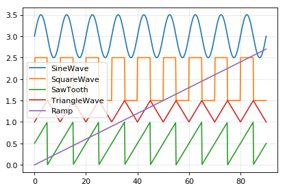
Generate different wave forms

Example for how to create different wave form functions in tellurium.

import tellurium as te
from roadrunner import Config

# We do not want CONSERVED MOIETIES set to true in this case
Config.setValue(Config.LOADSBMLOPTIONS_CONSERVED_MOIETIES, False)

# Generating different waveforms
model = '''
  model waveforms()
     # All waves have the following amplitude and period
     amplitude = 1
     period = 10

     # These events set the 'UpDown' variable to 1 or 0 according to the period.
     UpDown=0
     at sin(2*pi*time/period) >  0, t0=false: UpDown = 1
     at sin(2*pi*time/period) <= 0, t0=false: UpDown = 0

     # Simple Sine wave with y displaced by 3
     SineWave := amplitude/2*sin(2*pi*time/period) + 3

     # Square wave with y displaced by 1.5
     SquareWave := amplitude*UpDown + 1.5

     # Triangle waveform with given period and y displaced by 1
     TriangleWave = 1
     TriangleWave' = amplitude*2*(UpDown - 0.5)/period

     # Saw tooth wave form with given period
     SawTooth = amplitude/2
     SawTooth' = amplitude/period
     at UpDown==0: SawTooth = 0

     # Simple ramp
     Ramp := 0.03*time
  end
'''

r = te.loada(model)

r.timeCourseSelections = ['time', 'SineWave', 'SquareWave', 'SawTooth', 'TriangleWave', 'Ramp']
result = r.simulate (0, 90, 500)
r.plot(result)

# reset to default config
Config.setValue(Config.LOADSBMLOPTIONS_CONSERVED_MOIETIES, False)

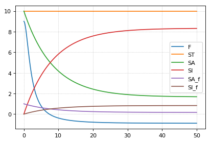
Normalized species

Example model which calculates functions depending on the normalized values of a species which can be either in active state SA or inactive state SI.

The normalized values are SA_f and SI_f, respectively, with the total concentration of S given as

ST = SA + SI

Model definition

The model is defined using Tellurium and Antimony. The identical equations could be typed directly in COPASI.

The created model is exported as SBML which than can be used in COPASI.

import tellurium as te
r = te.loada("""
    model normalized_species()

    # conversion between active (SA) and inactive (SI)
    J1: SA -> SI; k1*SA - k2*SI;
    k1 = 0.1; k2 = 0.02;

    # species
    species SA, SI, ST;
    SA = 10.0; SI = 0.0;
    const ST := SA + SI;

    SA is "active state S";
    SI is "inactive state S";
    ST is "total state S";

    # normalized species calculated via assignment rules
    species SA_f, SI_f;
    SA_f := SA/ST;
    SI_f := SI/ST;

    SA_f is "normalized active state S";
    SI_f is "normalized inactive state S";

    # parameters for your function
    P = 0.1;
    tau = 10.0;
    nA = 1.0;
    nI = 2.0;
    kA = 0.1;
    kI = 0.2;
    # now just use the normalized species in some math
    F := ( (1-(SI_f^nI)/(kI^nI+SI_f^nI)*(kI^nI+1) ) * ( (SA_f^nA)/(kA^nA+SA_f^nA)*(kA^nA+1) ) -P)*tau;

    end
""")
# print(r.getAntimony())

# Store the SBML for COPASI
import os
import tempfile
temp_dir = tempfile.mkdtemp()
file_path = os.path.join(temp_dir, 'normalizedSpecies.xml')
r.exportToSBML(file_path)

Model simulation

We perform a simple model simulation to demonstrate the main features using roadrunner: - normalized values SA_f and SI_f are normalized in [0,1] - the normalized values have same dynamics like SA and SF - the normalized values can be used to calculates some dependent function, here F

r.reset()
# select the variables of interest in output
r.selections = ['time', 'F'] + r.getBoundarySpeciesIds() \
                             + r.getFloatingSpeciesIds()
# simulate from 0 to 50 with 1001 points
s = r.simulate(0,50,1001)
# plot the results
r.plot(s);

Simulation and Analysis Methods

In this section, different ways to simlate and analyse a model is shown.

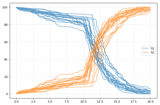
Stochastic simulations can be run by changing the current integrator type to ‘gillespie’ or by using the r.gillespie function.

import tellurium as te
import numpy as np

r = te.loada('S1 -> S2; k1*S1; k1 = 0.1; S1 = 40')
r.integrator = 'gillespie'
r.integrator.seed = 1234

results = []
for k in range(1, 50):
    r.reset()
    s = r.simulate(0, 40)
    results.append(s)
    r.plot(s, show=False, alpha=0.7)
te.show()

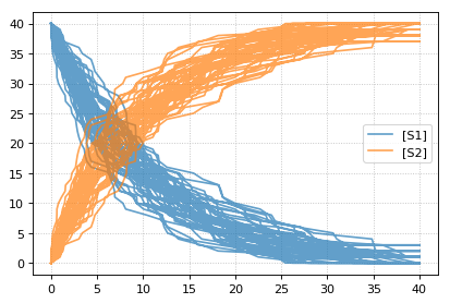
Setting the identical seed for all repeats results in identical traces in each simulation.

results = []
for k in range(1, 20):
    r.reset()
    r.setSeed(123456)
    s = r.simulate(0, 40)
    results.append(s)
    r.plot(s, show=False, loc=None, color='black', alpha=0.7)
te.show()

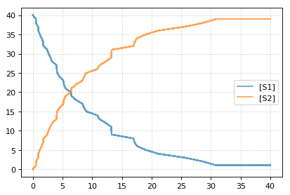
You can combine two timecourse simulations and change e.g. parameter values in between each simulation. The gillespie method simulates up to the given end time 10, after which you can make arbitrary changes to the model, then simulate again.

When using the r.plot function, you can pass the parameter labels, which controls the names that will be used in the figure legend, and tag, which ensures that traces with the same tag will be drawn with the same color (each species within each trace will be plotted in its own color, but these colors will match trace to trace).

import tellurium as te

r = te.loada('S1 -> S2; k1*S1; k1 = 0.02; S1 = 100')
r.setSeed(1234)
for k in range(1, 20):
    r.resetToOrigin()
    res1 = r.gillespie(0, 10)
    r.plot(res1, show=False) # plot first half of data

    # change in parameter after the first half of the simulation
    # We could have also used an Event in the antimony model,
    # which are described further in the Antimony Reference section
    r.k1 = r.k1*20
    res2 = r.gillespie (10, 20)

    r.plot(res2, show=False) # plot second half of data

te.show()

SED-ML

Tellurium exchangeability via the simulation experiment description markup language SED-ML and COMBINE archives (.omex files). These formats are designed to allow modeling software to exchange models and simulations. Whereas SBML encodes models, SED-ML encodes simulations, including the solver (e.g. deterministic or stochastic), the type of simulation (timecourse or steady state), and various parameters (start/end time, ODE solver tolerances, etc.).

Working with SED-ML

SED-ML describes how to run a set of simulations on a model encoded in SBML or CellML through specifying tasks, algorithm parameters, and post-processing. SED-ML has a limited vocabulary of simulation types (timecourse and steady state) is not designed to replace scripting with Python or other general-purpose languages. Instead, SED-ML is designed to provide a rudimentary way to reproduce the dynamics of a model across different tools. This process would otherwise require human intervention and becomes very laborious when thousands of models are involved.

The basic elements of a SED-ML document are:

• Models, which reference external SBML/CellML files or other previously defined models within the same SED-ML document,

• Simulations, which reference specific numerical solvers from the KiSAO ontology,

• Tasks, which apply a simulation to a model, and

• Outputs, which can be plots or reports.

Models in SED-ML essentially create instances of SBML/CellML models, and each instance can have different parameters.

Tellurium’s approach to handling SED-ML is to first convert the SED-ML document to a Python script, which contains all the Tellurium-specific function calls to run all tasks described in the SED-ML. For authoring SED-ML, Tellurium uses PhraSEDML, a human-readable analog of SED-ML. Example syntax is shown below.

SED-ML files are not very useful in isolation. Since SED-ML always references external SBML and CellML files, software which supports exchanging SED-ML files should use COMBINE archives, which package all related standards-encoded files together.

Reproducible computational biology experiments with SED-ML - The Simulation Experiment Description Markup Language. Waltemath D., Adams R., Bergmann F.T., Hucka M., Kolpakov F., Miller A.K., Moraru I.I., Nickerson D., Snoep J.L.,Le Novère, N. BMC Systems Biology 2011, 5:198 (http://www.pubmed.org/22172142)

Creating a SED-ML file

This example shows how to use PhraSEDML to author SED-ML files. Whenever a PhraSEDML script references an external model, you should use phrasedml.setReferencedSBML to ensure that the PhraSEDML script can be properly converted into a SED-ML file.

import tellurium as te
te.setDefaultPlottingEngine('matplotlib')
import phrasedml

antimony_str = '''
model myModel
  S1 -> S2; k1*S1
  S1 = 10; S2 = 0
  k1 = 1
end
'''

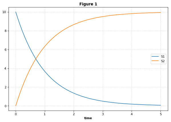
phrasedml_str = '''
  model1 = model "myModel"
  sim1 = simulate uniform(0, 5, 100)
  task1 = run sim1 on model1
  plot "Figure 1" time vs S1, S2
'''

# create the sedml xml string from the phrasedml
sbml_str = te.antimonyToSBML(antimony_str)
phrasedml.setReferencedSBML("myModel", sbml_str)

sedml_str = phrasedml.convertString(phrasedml_str)
if sedml_str == None:
    print(phrasedml.getLastPhrasedError())
print(sedml_str)

<?xml version="1.0" encoding="UTF-8"?>
<!-- Created by phraSED-ML version v1.0.9 with libSBML version 5.15.0. -->
<sedML xmlns="http://sed-ml.org/sed-ml/level1/version2" level="1" version="2">
  <listOfSimulations>
    <uniformTimeCourse id="sim1" initialTime="0" outputStartTime="0" outputEndTime="5" numberOfPoints="100">
      <algorithm kisaoID="KISAO:0000019"/>
    </uniformTimeCourse>
  </listOfSimulations>
  <listOfModels>
    <model id="model1" language="urn:sedml:language:sbml.level-3.version-1" source="myModel"/>
  </listOfModels>
  <listOfTasks>
    <task id="task1" modelReference="model1" simulationReference="sim1"/>
  </listOfTasks>
  <listOfDataGenerators>
    <dataGenerator id="plot_0_0_0" name="time">
      <listOfVariables>
        <variable id="time" symbol="urn:sedml:symbol:time" taskReference="task1"/>
      </listOfVariables>
      <math xmlns="http://www.w3.org/1998/Math/MathML">
        <ci> time </ci>
      </math>
    </dataGenerator>
    <dataGenerator id="plot_0_0_1" name="S1">
      <listOfVariables>
        <variable id="S1" target="/sbml:sbml/sbml:model/sbml:listOfSpecies/sbml:species[@id='S1']" taskReference="task1" modelReference="model1"/>
      </listOfVariables>
      <math xmlns="http://www.w3.org/1998/Math/MathML">
        <ci> S1 </ci>
      </math>
    </dataGenerator>
    <dataGenerator id="plot_0_1_1" name="S2">
      <listOfVariables>
        <variable id="S2" target="/sbml:sbml/sbml:model/sbml:listOfSpecies/sbml:species[@id='S2']" taskReference="task1" modelReference="model1"/>
      </listOfVariables>
      <math xmlns="http://www.w3.org/1998/Math/MathML">
        <ci> S2 </ci>
      </math>
    </dataGenerator>
  </listOfDataGenerators>
  <listOfOutputs>
    <plot2D id="plot_0" name="Figure 1">
      <listOfCurves>
        <curve id="plot_0__plot_0_0_0__plot_0_0_1" logX="false" logY="false" xDataReference="plot_0_0_0" yDataReference="plot_0_0_1"/>
        <curve id="plot_0__plot_0_0_0__plot_0_1_1" logX="false" logY="false" xDataReference="plot_0_0_0" yDataReference="plot_0_1_1"/>
      </listOfCurves>
    </plot2D>
  </listOfOutputs>
</sedML>

Reading / Executing SED-ML

After converting PhraSEDML to SED-ML, you can call te.executeSEDML to use Tellurium to execute all simulations in the SED-ML. This example also shows how to use libSEDML (used by Tellurium and PhraSEDML internally) for reading SED-ML files.

import tempfile, os, shutil

workingDir = tempfile.mkdtemp(suffix="_sedml")

sbml_file = os.path.join(workingDir, 'myModel')
sedml_file = os.path.join(workingDir, 'sed_main.xml')

with open(sbml_file, 'wb') as f:
    f.write(sbml_str.encode('utf-8'))
    f.flush()
    print('SBML written to temporary file')

with open(sedml_file, 'wb') as f:
    f.write(sedml_str.encode('utf-8'))
    f.flush()
    print('SED-ML written to temporary file')

# For technical reasons, any software which uses libSEDML
# must provide a custom build - Tellurium uses tesedml
try:
    import libsedml
except ImportError:
    import tesedml as libsedml
sedml_doc = libsedml.readSedML(sedml_file)
n_errors = sedml_doc.getErrorLog().getNumFailsWithSeverity(libsedml.LIBSEDML_SEV_ERROR)
print('Read SED-ML file, number of errors: {}'.format(n_errors))
if n_errors > 0:
    print(sedml_doc.getErrorLog().toString())

# execute SED-ML using Tellurium
te.executeSEDML(sedml_str, workingDir=workingDir)

# clean up
#shutil.rmtree(workingDir)

SBML written to temporary file
SED-ML written to temporary file
Read SED-ML file, number of errors: 0

SED-ML L1V2 specification example

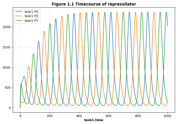
This example uses the celebrated repressilator model to demonstrate how to 1) download a model from the BioModels database, 2) create a PhraSEDML string to simulate the model, 3) convert the PhraSEDML to SED-ML, and 4) use Tellurium to execute the resulting SED-ML.

This and other examples here are the SED-ML reference specification (Introduction section).

import tellurium as te, tellurium.temiriam as temiriam
te.setDefaultPlottingEngine('matplotlib')
import phrasedml

# Get SBML from URN and set for phrasedml
urn = "urn:miriam:biomodels.db:BIOMD0000000012"
sbml_str = temiriam.getSBMLFromBiomodelsURN(urn=urn)
phrasedml.setReferencedSBML('BIOMD0000000012', sbml_str)

# <SBML species>
#   PX - LacI protein
#   PY - TetR protein
#   PZ - cI protein
#   X - LacI mRNA
#   Y - TetR mRNA
#   Z - cI mRNA

# <SBML parameters>
#   ps_a - tps_active: Transcrition from free promotor in transcripts per second and promotor
#   ps_0 - tps_repr: Transcrition from fully repressed promotor in transcripts per second and promotor

phrasedml_str = """
    model1 = model "{}"
    model2 = model model1 with ps_0=1.3E-5, ps_a=0.013
    sim1 = simulate uniform(0, 1000, 1000)
    task1 = run sim1 on model1
    task2 = run sim1 on model2

    # A simple timecourse simulation
    plot "Figure 1.1 Timecourse of repressilator" task1.time vs task1.PX, task1.PZ, task1.PY

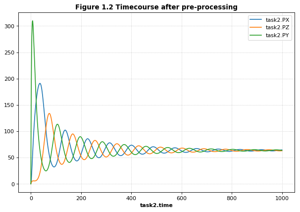
    # Applying preprocessing
    plot "Figure 1.2 Timecourse after pre-processing" task2.time vs task2.PX, task2.PZ, task2.PY

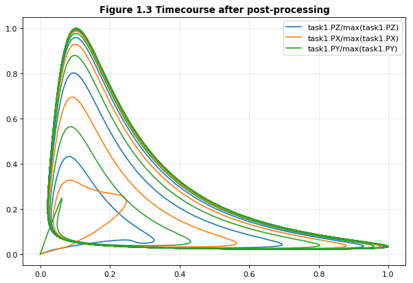
    # Applying postprocessing
    plot "Figure 1.3 Timecourse after post-processing" task1.PX/max(task1.PX) vs task1.PZ/max(task1.PZ), \
                                                       task1.PY/max(task1.PY) vs task1.PX/max(task1.PX), \
                                                       task1.PZ/max(task1.PZ) vs task1.PY/max(task1.PY)
""".format('BIOMD0000000012')

# convert to SED-ML
sedml_str = phrasedml.convertString(phrasedml_str)
if sedml_str == None:
    raise RuntimeError(phrasedml.getLastError())

# Run the SED-ML file with results written in workingDir
import tempfile, shutil, os
workingDir = tempfile.mkdtemp(suffix="_sedml")
# write out SBML
with open(os.path.join(workingDir, 'BIOMD0000000012'), 'wb') as f:
    f.write(sbml_str.encode('utf-8'))
te.executeSEDML(sedml_str, workingDir=workingDir)
shutil.rmtree(workingDir)

COMBINE & Inline OMEX

COMBINE archives package related standards such as SBML models and SED-ML simulations together so that they can be easily exchanged between software tools. Tellurium provides the inline OMEX format for editing the contents of COMBINE archives in a human-readable format. You can use the function convertCombineArchive to convert a COMBINE archive on disk to an inline OMEX string, and the function executeInlineOmex to execute the inline OMEX string. Examples below.

tellurium.convertCombineArchive(location)

Read a COMBINE archive and convert its contents to an inline Omex.

Parameters:

location – Filesystem path to the archive.

tellurium.executeInlineOmex(inline_omex, comp=False)

Execute inline phrasedml and antimony.

Parameters:

inline_omex – String containing inline phrasedml and antimony.

tellurium.exportInlineOmex(inline_omex, export_location)

Export an inline OMEX string to a COMBINE archive.

Parameters:

• inline_omex – String containing inline OMEX describing models and simulations.

• export_location – Filepath of Combine archive to create.

tellurium.extractFileFromCombineArchive(archive_path, entry_location)

Extract a single file from a COMBINE archive and return it as a string.

Inline OMEX and COMBINE archives

Tellurium provides a way to easily edit the contents of COMBINE archives in a human-readable format called inline OMEX. To create a COMBINE archive, simply create a string containing all models (in Antimony format) and all simulations (in PhraSEDML format). Tellurium will transparently convert the Antimony to SBML and PhraSEDML to SED-ML, then execute the resulting SED-ML. The following example will work in either Jupyter or the Tellurium notebook viewer. The Tellurium notebook viewer allows you to create specialized cells for inline OMEX, which contain correct syntax-highlighting for the format.

import tellurium as te, tempfile, os
te.setDefaultPlottingEngine('matplotlib')

antimony_str = '''
model myModel
  S1 -> S2; k1*S1
  S1 = 10; S2 = 0
  k1 = 1
end
'''

phrasedml_str = '''
  model1 = model "myModel"
  sim1 = simulate uniform(0, 5, 100)
  task1 = run sim1 on model1
  plot "Figure 1" time vs S1, S2
'''

# create an inline OMEX (inline representation of a COMBINE archive)
# from the antimony and phrasedml strings
inline_omex = '\n'.join([antimony_str, phrasedml_str])

# execute the inline OMEX
te.executeInlineOmex(inline_omex)
# export to a COMBINE archive
workingDir = tempfile.mkdtemp(suffix="_omex")
te.exportInlineOmex(inline_omex, os.path.join(workingDir, 'archive.omex'))

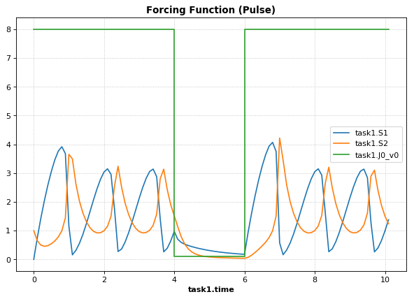
Forcing Functions

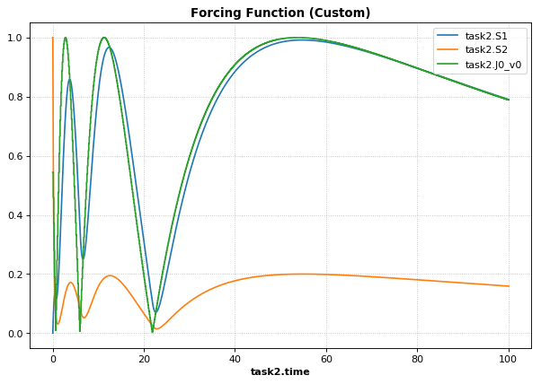
A common task in modeling is to represent the influence of an external, time-varying input on the system. In SED-ML, this can be accomplished using a repeated task to run a simulation for a short amount of time and update the forcing function between simulations. In the example, the forcing function is a pulse represented with a piecewise directive, but it can be any arbitrarily complex time-varying function, as shown in the second example.

import tellurium as te

antimony_str = '''
// Created by libAntimony v2.9
model *oneStep()

// Compartments and Species:
compartment compartment_;
species S1 in compartment_, S2 in compartment_, $X0 in compartment_, $X1 in compartment_;
species $X2 in compartment_;

// Reactions:
J0: $X0 => S1; J0_v0;
J1: S1 => $X1; J1_k3*S1;
J2: S1 => S2; (J2_k1*S1 - J2_k_1*S2)*(1 + J2_c*S2^J2_q);
J3: S2 => $X2; J3_k2*S2;

// Species initializations:
S1 = 0;
S2 = 1;
X0 = 1;
X1 = 0;
X2 = 0;

// Compartment initializations:
compartment_ = 1;

// Variable initializations:
J0_v0 = 8;
J1_k3 = 0;
J2_k1 = 1;
J2_k_1 = 0;
J2_c = 1;
J2_q = 3;
J3_k2 = 5;

// Other declarations:
const compartment_, J0_v0, J1_k3, J2_k1, J2_k_1, J2_c, J2_q, J3_k2;
end
'''

phrasedml_str = '''
model1 = model "oneStep"
stepper = simulate onestep(0.1)
task0 = run stepper on model1
task1 = repeat task0 for local.x in uniform(0, 10, 100), J0_v0 = piecewise(8, x<4, 0.1, 4<=x<6, 8)
task2 = repeat task0 for local.index in uniform(0, 10, 1000), local.current = index -> abs(sin(1 / (0.1 * index + 0.1))), model1.J0_v0 = current : current
plot "Forcing Function (Pulse)" task1.time vs task1.S1, task1.S2, task1.J0_v0
plot "Forcing Function (Custom)" task2.time vs task2.S1, task2.S2, task2.J0_v0
'''

# create the inline OMEX string
inline_omex = '\n'.join([antimony_str, phrasedml_str])

# export to a COMBINE archive
workingDir = tempfile.mkdtemp(suffix="_omex")
archive_name = os.path.join(workingDir, 'archive.omex')
te.exportInlineOmex(inline_omex, archive_name)
# convert the COMBINE archive back into an
# inline OMEX (transparently) and execute it
te.convertAndExecuteCombineArchive(archive_name)

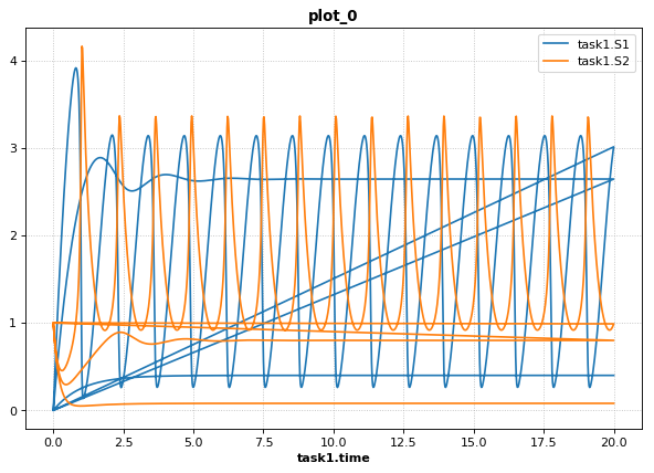
1d Parameter Scan

This example shows how to perform a one-dimensional parameter scan using Antimony/PhraSEDML and convert the study to a COMBINE archive. The example uses a PhraSEDML repeated task task1 to run a timecourse simulation task0 on a model for different values of the parameter J0_v0.

import tellurium as te

antimony_str = '''
// Created by libAntimony v2.9
model *parameterScan1D()

// Compartments and Species:
compartment compartment_;
species S1 in compartment_, S2 in compartment_, $X0 in compartment_, $X1 in compartment_;
species $X2 in compartment_;

// Reactions:
J0: $X0 => S1; J0_v0;
J1: S1 => $X1; J1_k3*S1;
J2: S1 => S2; (J2_k1*S1 - J2_k_1*S2)*(1 + J2_c*S2^J2_q);
J3: S2 => $X2; J3_k2*S2;

// Species initializations:
S1 = 0;
S2 = 1;
X0 = 1;
X1 = 0;
X2 = 0;

// Compartment initializations:
compartment_ = 1;

// Variable initializations:
J0_v0 = 8;
J1_k3 = 0;
J2_k1 = 1;
J2_k_1 = 0;
J2_c = 1;
J2_q = 3;
J3_k2 = 5;

// Other declarations:
const compartment_, J0_v0, J1_k3, J2_k1, J2_k_1, J2_c, J2_q, J3_k2;
end
'''

phrasedml_str = '''
model1 = model "parameterScan1D"
timecourse1 = simulate uniform(0, 20, 1000)
task0 = run timecourse1 on model1
task1 = repeat task0 for J0_v0 in [8, 4, 0.4], reset=true
plot task1.time vs task1.S1, task1.S2
'''

# create the inline OMEX string
inline_omex = '\n'.join([antimony_str, phrasedml_str])

# execute the inline OMEX
te.executeInlineOmex(inline_omex)

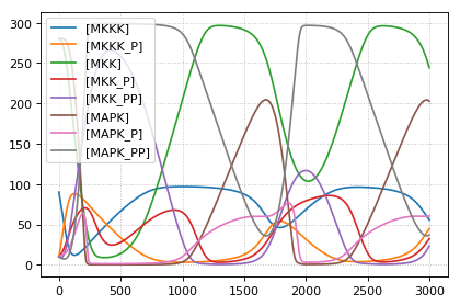
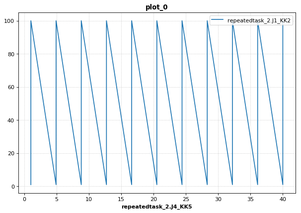
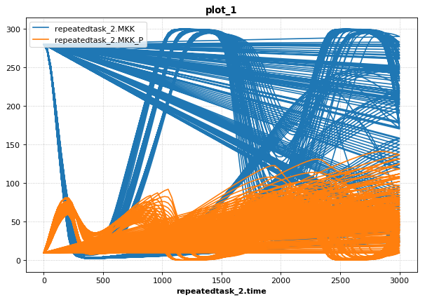
2d Parameter Scan

There are multiple was to specify the set of values that should be swept over. This example uses two repeated tasks instead of one. It sweeps through a discrete set of values for the parameter J1_KK2, and then sweeps through a uniform range for another parameter J4_KK5.

import tellurium as te

antimony_str = '''
// Created by libAntimony v2.9
model *parameterScan2D()

  // Compartments and Species:
  compartment compartment_;
  species MKKK in compartment_, MKKK_P in compartment_, MKK in compartment_;
  species MKK_P in compartment_, MKK_PP in compartment_, MAPK in compartment_;
  species MAPK_P in compartment_, MAPK_PP in compartment_;

  // Reactions:
  J0: MKKK => MKKK_P; (J0_V1*MKKK)/((1 + (MAPK_PP/J0_Ki)^J0_n)*(J0_K1 + MKKK));
  J1: MKKK_P => MKKK; (J1_V2*MKKK_P)/(J1_KK2 + MKKK_P);
  J2: MKK => MKK_P; (J2_k3*MKKK_P*MKK)/(J2_KK3 + MKK);
  J3: MKK_P => MKK_PP; (J3_k4*MKKK_P*MKK_P)/(J3_KK4 + MKK_P);
  J4: MKK_PP => MKK_P; (J4_V5*MKK_PP)/(J4_KK5 + MKK_PP);
  J5: MKK_P => MKK; (J5_V6*MKK_P)/(J5_KK6 + MKK_P);
  J6: MAPK => MAPK_P; (J6_k7*MKK_PP*MAPK)/(J6_KK7 + MAPK);
  J7: MAPK_P => MAPK_PP; (J7_k8*MKK_PP*MAPK_P)/(J7_KK8 + MAPK_P);
  J8: MAPK_PP => MAPK_P; (J8_V9*MAPK_PP)/(J8_KK9 + MAPK_PP);
  J9: MAPK_P => MAPK; (J9_V10*MAPK_P)/(J9_KK10 + MAPK_P);

  // Species initializations:
  MKKK = 90;
  MKKK_P = 10;
  MKK = 280;
  MKK_P = 10;
  MKK_PP = 10;
  MAPK = 280;
  MAPK_P = 10;
  MAPK_PP = 10;

  // Compartment initializations:
  compartment_ = 1;

  // Variable initializations:
  J0_V1 = 2.5;
  J0_Ki = 9;
  J0_n = 1;
  J0_K1 = 10;
  J1_V2 = 0.25;
  J1_KK2 = 8;
  J2_k3 = 0.025;
  J2_KK3 = 15;
  J3_k4 = 0.025;
  J3_KK4 = 15;
  J4_V5 = 0.75;
  J4_KK5 = 15;
  J5_V6 = 0.75;
  J5_KK6 = 15;
  J6_k7 = 0.025;
  J6_KK7 = 15;
  J7_k8 = 0.025;
  J7_KK8 = 15;
  J8_V9 = 0.5;
  J8_KK9 = 15;
  J9_V10 = 0.5;
  J9_KK10 = 15;

  // Other declarations:
  const compartment_, J0_V1, J0_Ki, J0_n, J0_K1, J1_V2, J1_KK2, J2_k3, J2_KK3;
  const J3_k4, J3_KK4, J4_V5, J4_KK5, J5_V6, J5_KK6, J6_k7, J6_KK7, J7_k8;
  const J7_KK8, J8_V9, J8_KK9, J9_V10, J9_KK10;
end
'''

phrasedml_str = '''
  model_3 = model "parameterScan2D.xml"
  sim_repeat = simulate uniform(0,3000,100)
  task_1 = run sim_repeat on model_3
  repeatedtask_1 = repeat task_1 for J1_KK2 in [1, 5, 10, 50, 60, 70, 80, 90, 100], reset=true
  repeatedtask_2 = repeat repeatedtask_1 for J4_KK5 in uniform(1, 40, 10), reset=true
  plot repeatedtask_2.J4_KK5 vs repeatedtask_2.J1_KK2
  plot repeatedtask_2.time vs repeatedtask_2.MKK, repeatedtask_2.MKK_P
'''

# create the inline OMEX string
inline_omex = '\n'.join([antimony_str, phrasedml_str])

# execute the inline OMEX
te.executeInlineOmex(inline_omex)

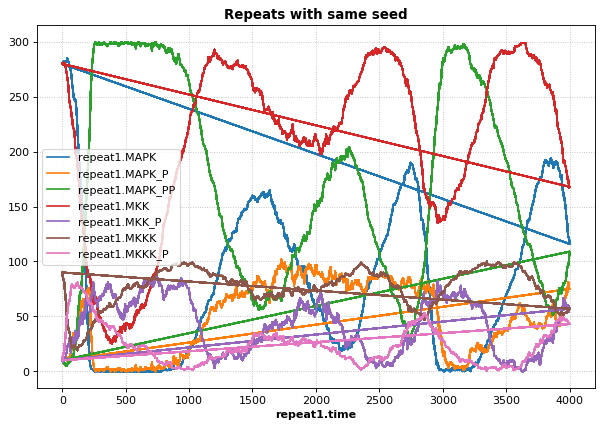
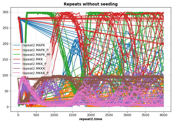
Stochastic Simulation and RNG Seeding

It is possible to programatically set the RNG seed of a stochastic simulation in PhraSEDML using the <simulation-name>.algorithm.seed = <value> directive. Simulations run with the same seed are identical. If the seed is not specified, a different value is used each time, leading to different results.

# -*- coding: utf-8 -*-
"""
phrasedml repeated stochastic test
"""
import tellurium as te

antimony_str = '''
// Created by libAntimony v2.9
model *repeatedStochastic()

// Compartments and Species:
compartment compartment_;
species MKKK in compartment_, MKKK_P in compartment_, MKK in compartment_;
species MKK_P in compartment_, MKK_PP in compartment_, MAPK in compartment_;
species MAPK_P in compartment_, MAPK_PP in compartment_;

// Reactions:
J0: MKKK => MKKK_P; (J0_V1*MKKK)/((1 + (MAPK_PP/J0_Ki)^J0_n)*(J0_K1 + MKKK));
J1: MKKK_P => MKKK; (J1_V2*MKKK_P)/(J1_KK2 + MKKK_P);
J2: MKK => MKK_P; (J2_k3*MKKK_P*MKK)/(J2_KK3 + MKK);
J3: MKK_P => MKK_PP; (J3_k4*MKKK_P*MKK_P)/(J3_KK4 + MKK_P);
J4: MKK_PP => MKK_P; (J4_V5*MKK_PP)/(J4_KK5 + MKK_PP);
J5: MKK_P => MKK; (J5_V6*MKK_P)/(J5_KK6 + MKK_P);
J6: MAPK => MAPK_P; (J6_k7*MKK_PP*MAPK)/(J6_KK7 + MAPK);
J7: MAPK_P => MAPK_PP; (J7_k8*MKK_PP*MAPK_P)/(J7_KK8 + MAPK_P);
J8: MAPK_PP => MAPK_P; (J8_V9*MAPK_PP)/(J8_KK9 + MAPK_PP);
J9: MAPK_P => MAPK; (J9_V10*MAPK_P)/(J9_KK10 + MAPK_P);

// Species initializations:
MKKK = 90;
MKKK_P = 10;
MKK = 280;
MKK_P = 10;
MKK_PP = 10;
MAPK = 280;
MAPK_P = 10;
MAPK_PP = 10;

// Compartment initializations:
compartment_ = 1;

// Variable initializations:
J0_V1 = 2.5;
J0_Ki = 9;
J0_n = 1;
J0_K1 = 10;
J1_V2 = 0.25;
J1_KK2 = 8;
J2_k3 = 0.025;
J2_KK3 = 15;
J3_k4 = 0.025;
J3_KK4 = 15;
J4_V5 = 0.75;
J4_KK5 = 15;
J5_V6 = 0.75;
J5_KK6 = 15;
J6_k7 = 0.025;
J6_KK7 = 15;
J7_k8 = 0.025;
J7_KK8 = 15;
J8_V9 = 0.5;
J8_KK9 = 15;
J9_V10 = 0.5;
J9_KK10 = 15;

// Other declarations:
const compartment_, J0_V1, J0_Ki, J0_n, J0_K1, J1_V2, J1_KK2, J2_k3, J2_KK3;
const J3_k4, J3_KK4, J4_V5, J4_KK5, J5_V6, J5_KK6, J6_k7, J6_KK7, J7_k8;
const J7_KK8, J8_V9, J8_KK9, J9_V10, J9_KK10;
end
'''

phrasedml_str = '''
model1 = model "repeatedStochastic"
timecourse1 = simulate uniform_stochastic(0, 4000, 1000)
timecourse1.algorithm.seed = 1003
timecourse2 = simulate uniform_stochastic(0, 4000, 1000)
task1 = run timecourse1 on model1
task2 = run timecourse2 on model1
repeat1 = repeat task1 for local.x in uniform(0, 10, 10), reset=true
repeat2 = repeat task2 for local.x in uniform(0, 10, 10), reset=true
plot "Repeats with same seed" repeat1.time vs repeat1.MAPK, repeat1.MAPK_P, repeat1.MAPK_PP, repeat1.MKK, repeat1.MKK_P, repeat1.MKKK, repeat1.MKKK_P
plot "Repeats without seeding" repeat2.time vs repeat2.MAPK, repeat2.MAPK_P, repeat2.MAPK_PP, repeat2.MKK, repeat2.MKK_P, repeat2.MKKK, repeat2.MKKK_P
'''

# create the inline OMEX string
inline_omex = '\n'.join([antimony_str, phrasedml_str])

# execute the inline OMEX
te.executeInlineOmex(inline_omex)

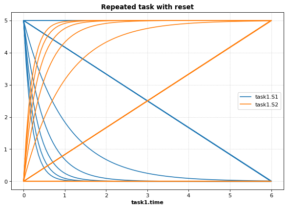
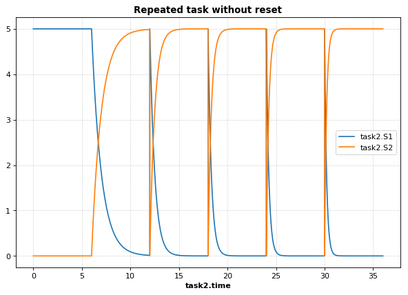
Resetting Models

This example is another parameter scan which shows the effect of resetting the model or not after each simulation. When using the repeated task directive in PhraSEDML, you can pass the reset=true argument to reset the model to its initial conditions after each repeated simulation. Leaving this argument off causes the model to retain its current state between simulations. In this case, the time value is not reset.

import tellurium as te

antimony_str = """
model case_02
    J0: S1 -> S2; k1*S1;
    S1 = 10.0; S2=0.0;
    k1 = 0.1;
end
"""

phrasedml_str = """
    model0 = model "case_02"
    model1 = model model0 with S1=5.0
    sim0 = simulate uniform(0, 6, 100)
    task0 = run sim0 on model1
    # reset the model after each simulation
    task1 = repeat task0 for k1 in uniform(0.0, 5.0, 5), reset = true
    # show the effect of not resetting for comparison
    task2 = repeat task0 for k1 in uniform(0.0, 5.0, 5)
    plot "Repeated task with reset"    task1.time vs task1.S1, task1.S2
    plot "Repeated task without reset" task2.time vs task2.S1, task2.S2
"""

# create the inline OMEX string
inline_omex = '\n'.join([antimony_str, phrasedml_str])

# execute the inline OMEX
te.executeInlineOmex(inline_omex)

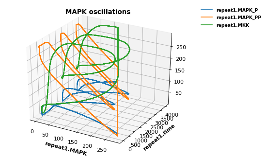
3d Plotting

This example shows how to use PhraSEDML to perform 3d plotting. The syntax is plot <x> vs <y> vs <z>, where <x>, <y>, and <z> are references to model state variables used in specific tasks.

import tellurium as te

antimony_str = '''
// Created by libAntimony v2.9
model *case_09()

// Compartments and Species:
compartment compartment_;
species MKKK in compartment_, MKKK_P in compartment_, MKK in compartment_;
species MKK_P in compartment_, MKK_PP in compartment_, MAPK in compartment_;
species MAPK_P in compartment_, MAPK_PP in compartment_;

// Reactions:
J0: MKKK => MKKK_P; (J0_V1*MKKK)/((1 + (MAPK_PP/J0_Ki)^J0_n)*(J0_K1 + MKKK));
J1: MKKK_P => MKKK; (J1_V2*MKKK_P)/(J1_KK2 + MKKK_P);
J2: MKK => MKK_P; (J2_k3*MKKK_P*MKK)/(J2_KK3 + MKK);
J3: MKK_P => MKK_PP; (J3_k4*MKKK_P*MKK_P)/(J3_KK4 + MKK_P);
J4: MKK_PP => MKK_P; (J4_V5*MKK_PP)/(J4_KK5 + MKK_PP);
J5: MKK_P => MKK; (J5_V6*MKK_P)/(J5_KK6 + MKK_P);
J6: MAPK => MAPK_P; (J6_k7*MKK_PP*MAPK)/(J6_KK7 + MAPK);
J7: MAPK_P => MAPK_PP; (J7_k8*MKK_PP*MAPK_P)/(J7_KK8 + MAPK_P);
J8: MAPK_PP => MAPK_P; (J8_V9*MAPK_PP)/(J8_KK9 + MAPK_PP);
J9: MAPK_P => MAPK; (J9_V10*MAPK_P)/(J9_KK10 + MAPK_P);

// Species initializations:
MKKK = 90;
MKKK_P = 10;
MKK = 280;
MKK_P = 10;
MKK_PP = 10;
MAPK = 280;
MAPK_P = 10;
MAPK_PP = 10;

// Compartment initializations:
compartment_ = 1;

// Variable initializations:
J0_V1 = 2.5;
J0_Ki = 9;
J0_n = 1;
J0_K1 = 10;
J1_V2 = 0.25;
J1_KK2 = 8;
J2_k3 = 0.025;
J2_KK3 = 15;
J3_k4 = 0.025;
J3_KK4 = 15;
J4_V5 = 0.75;
J4_KK5 = 15;
J5_V6 = 0.75;
J5_KK6 = 15;
J6_k7 = 0.025;
J6_KK7 = 15;
J7_k8 = 0.025;
J7_KK8 = 15;
J8_V9 = 0.5;
J8_KK9 = 15;
J9_V10 = 0.5;
J9_KK10 = 15;

// Other declarations:
const compartment_, J0_V1, J0_Ki, J0_n, J0_K1, J1_V2, J1_KK2, J2_k3, J2_KK3;
const J3_k4, J3_KK4, J4_V5, J4_KK5, J5_V6, J5_KK6, J6_k7, J6_KK7, J7_k8;
const J7_KK8, J8_V9, J8_KK9, J9_V10, J9_KK10;
end
'''

phrasedml_str = '''
  mod1 = model "case_09"
  # sim1 = simulate uniform_stochastic(0, 4000, 1000)
  sim1 = simulate uniform(0, 4000, 1000)
  task1 = run sim1 on mod1
  repeat1 = repeat task1 for local.x in uniform(0, 10, 10), reset=true
  plot "MAPK oscillations" repeat1.MAPK vs repeat1.time vs repeat1.MAPK_P, repeat1.MAPK vs repeat1.time vs repeat1.MAPK_PP, repeat1.MAPK vs repeat1.time vs repeat1.MKK
  # report repeat1.MAPK vs repeat1.time vs repeat1.MAPK_P, repeat1.MAPK vs repeat1.time vs repeat1.MAPK_PP, repeat1.MAPK vs repeat1.time vs repeat1.MKK
'''

# create the inline OMEX string
inline_omex = '\n'.join([antimony_str, phrasedml_str])

# execute the inline OMEX
te.executeInlineOmex(inline_omex)

Modeling Case Studies

This series of case studies shows some slight more advanced examples which correspond to common motifs in biological networks (negative feedback loops, etc.). To draw the network diagrams seen here, you will need graphviz installed.

Preliminaries

In order to draw the network graphs in these examples (i.e. using r.draw()), you will need graphviz and pygraphviz installed. Please consult the Graphviz documentation for instructions on installing it on your platform. If you cannot install Graphviz and yraphviz, you can still run the following examples, but the network diagrams will not be generated.

Also, due to limitations in pygraphviz, these examples can only be run in the Jupyter notebook, not the Tellurium notebook app.

Install pygraphviz (requires compilation)

Please run

<your-local-python-executable> -m pip install pygraphviz

from a terminal or command prompt to install pygraphviz. Then restart your kernel in this notebook (Language->Restart Running Kernel).

Troubleshooting Graphviz Installation

pygraphviz has known problems during installation on some platforms. On 64-bit Fedora Linux, we have been able to use the following command to install pygraphviz:

/path/to/python3 -m pip install pygraphviz --install-option="--include-path=/usr/include/graphviz" --install-option="--library-path=/usr/lib64/graphviz/"

You may need to modify the library/include paths in the above command. Some Linux distributions put 64-bit libraries in /usr/lib instead of /usr/lib64, in which case the command becomes:

/path/to/python3 -m pip install pygraphviz --install-option="--include-path=/usr/include/graphviz" --install-option="--library-path=/usr/lib/graphviz/"

Case Studies

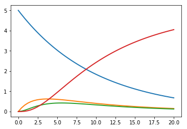
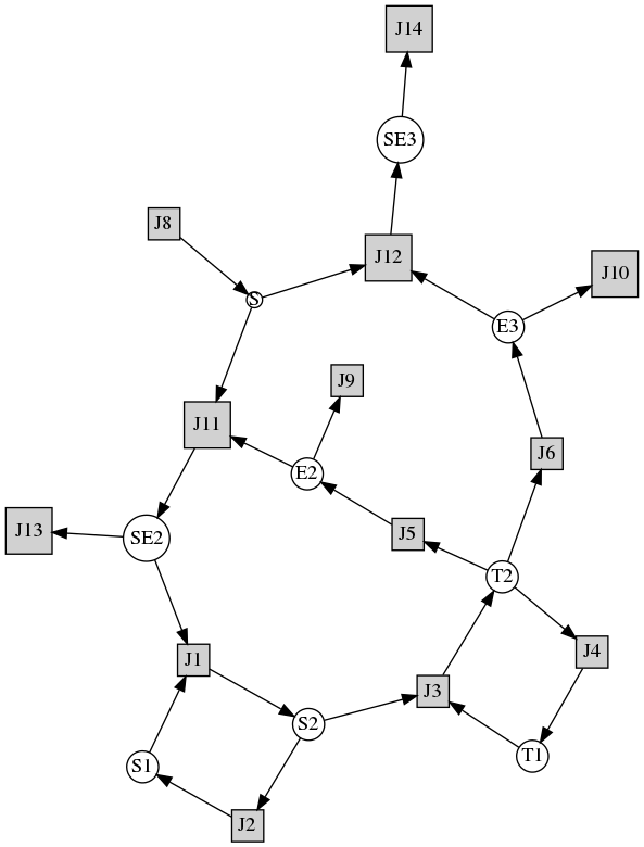
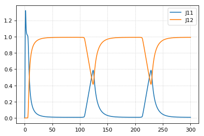
Activator system

import warnings
warnings.filterwarnings("ignore")

import tellurium as te
te.setDefaultPlottingEngine('matplotlib')

# model Definition
r = te.loada ('''
        #J1: S1 -> S2; Activator*kcat1*S1/(Km1+S1);
        J1: S1 -> S2; SE2*kcat1*S1/(Km1+S1);
        J2: S2 -> S1; Vm2*S2/(Km2+S2);

        J3: T1 -> T2; S2*kcat3*T1/(Km3+T1);
        J4: T2 -> T1; Vm4*T2/(Km4+T2);

        J5:    -> E2; Vf5/(Ks5+T2^h5);
        J6:    -> E3; Vf6*T2^h6/(Ks6+T2^h6);

        #J7:    -> E1;
        J8:    ->  S; kcat8*E1

        J9: E2 ->   ; k9*E2;
        J10:E3 ->   ; k10*E3;

        J11: S -> SE2; E2*kcat11*S/(Km11+S);
        J12: S -> SE3; E3*kcat12*S/(Km12+S);

        J13: SE2 ->  ; SE2*kcat13;
        J14: SE3 ->  ; SE3*kcat14;

        Km1 = 0.01; Km2 = 0.01; Km3 = 0.01; Km4 = 0.01; Km11 = 1; Km12 = 0.1;
        S1 = 6; S2 =0.1; T1=6; T2 = 0.1;
        SE2 = 0; SE3=0;
        S=0;
        E2 = 0; E3 = 0;
        kcat1 = 0.1; kcat3 = 3; kcat8 =1; kcat11 = 1; kcat12 = 1; kcat13 = 0.1; kcat14=0.1;
        E1 = 1;
        k9 = 0.1; k10=0.1;
        Vf6 = 1;
        Vf5 = 3;
        Vm2 = 0.1;
        Vm4 = 2;
        h6 = 2; h5=2;
        Ks6 = 1; Ks5 = 1;
        Activator = 0;

        at (time > 100): Activator = 5;
''')
r.draw(width=300)
result = r.simulate (0, 300, 2000, ['time', 'J11', 'J12']);
r.plot(result);

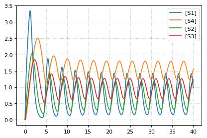
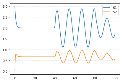
Feedback oscillations

# http://tellurium.analogmachine.org/testing/
import tellurium as te
r = te.loada ('''
model feedback()
   // Reactions:
   J0: $X0 -> S1; (VM1 * (X0 - S1/Keq1))/(1 + X0 + S1 +   S4^h);
   J1: S1 -> S2; (10 * S1 - 2 * S2) / (1 + S1 + S2);
   J2: S2 -> S3; (10 * S2 - 2 * S3) / (1 + S2 + S3);
   J3: S3 -> S4; (10 * S3 - 2 * S4) / (1 + S3 + S4);
   J4: S4 -> $X1; (V4 * S4) / (KS4 + S4);

  // Species initializations:
  S1 = 0; S2 = 0; S3 = 0;
  S4 = 0; X0 = 10; X1 = 0;

  // Variable initialization:
  VM1 = 10; Keq1 = 10; h = 10; V4 = 2.5; KS4 = 0.5;
end''')

r.integrator.setValue('variable_step_size', True)
res = r.simulate(0, 40)
r.plot()

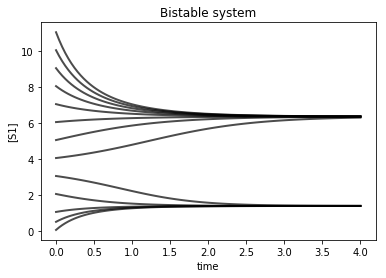
Bistable System

Example showing how to to multiple time course simulations, merging the data and plotting it onto one plotting surface. Alternative is to use setHold()

Model is a bistable system, simulations start with different initial conditions resulting in different steady states reached.

import tellurium as te
import numpy as np

r = te.loada ('''
$Xo -> S1; 1 + Xo*(32+(S1/0.75)^3.2)/(1 +(S1/4.3)^3.2);
S1 -> $X1; k1*S1;

Xo = 0.09; X1 = 0.0;
S1 = 0.5; k1 = 3.2;
''')
print(r.selections)

initValue = 0.05
m = r.simulate (0, 4, 100, selections=["time", "[S1]"])

for i in range (0,12):
    r.reset()
    r['[S1]'] = initValue
    res = r.simulate (0, 4, 100, selections=["[S1]"])
    m = np.concatenate([m, res], axis=1)
    initValue += 1

te.plotArray(m, color="black", alpha=0.7, loc=None,
             xlabel="time", ylabel="[S1]", title="Bistable system");

['time', '[S1]']

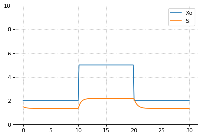
Events

import tellurium as te
import matplotlib.pyplot as plt

# Example showing use of events and how to set the y axis limits
r = te.loada ('''
  $Xo -> S;   Xo/(km + S^h);
  S -> $w;  k1*S;

     # initialize
     h = 1;   # Hill coefficient
     k1 = 1;  km = 0.1;
     S = 1.5; Xo = 2

     at (time > 10): Xo = 5;
     at (time > 20): Xo = 2;
''')

m1 = r.simulate (0, 30, 200, ['time', 'Xo', 'S'])
r.plot(ylim=(0,10))

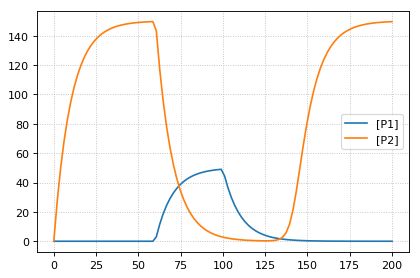
Gene network

import tellurium as te
import numpy

# Model describes a cascade of two genes. First gene is activated
# second gene is repressed. Uses events to change the input
# to the gene regulatory network

r = te.loada ('''
    v1:  -> P1; Vm1*I^4/(Km1 + I^4);
    v2:  P1 -> ; k1*P1;
    v3:  -> P2;  Vm2/(Km2 + P1^4);
    v4:  P2 -> ; k2*P2;

    at (time > 60): I = 10;
    at (time > 100): I = 0.01;
    Vm1  = 5; Vm2 = 6; Km1 = 0.5; Km2 = 0.4;
    k1 = 0.1; k2 = 0.1;
    I = 0.01;
''')

result = r.simulate (0, 200, 100)
r.plot()

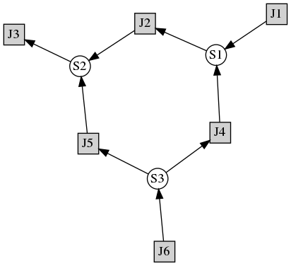
Stoichiometric matrix

import tellurium as te

# Example of using antimony to create a stoichiometry matrix
r = te.loada('''
 J1: -> S1; v1;
 J2: S1 -> S2; v2;
 J3: S2 -> ; v3;
 J4: S3 -> S1; v4;
 J5: S3 -> S2; v5;
 J6: -> S3; v6;

 v1=1; v2=1; v3=1; v4=1; v5=1; v6=1;
''')

print(r.getFullStoichiometryMatrix())
r.draw()

      J1, J2, J3, J4, J5, J6
S1 [[  1, -1,  0,  1,  0,  0],
S2  [  0,  1, -1,  0,  1,  0],
S3  [  0,  0,  0, -1, -1,  1]]

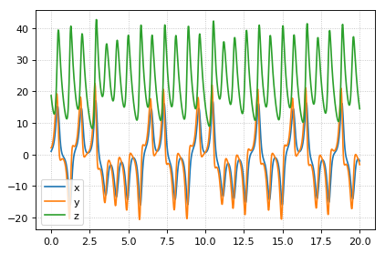
Lorenz attractor

Example showing how to describe a model using ODES. Example implements the Lorenz attractor.

import tellurium as te

r = te.loada ('''
     x' = sigma*(y - x);
     y' = x*(rho - z) - y;
     z' = x*y - beta*z;

     x = 0.96259;  y = 2.07272;  z = 18.65888;

     sigma = 10;  rho = 28; beta = 2.67;
''')

result = r.simulate (0, 20, 1000, ['time', 'x', 'y', 'z'])
r.plot()

Time Course Parameter Scan

Do 5 simulations on a simple model, for each simulation a parameter, k1 is changed. The script merges the data together and plots the merged array on to one plot.

import tellurium as te
import numpy as np

r = te.loada ('''
    J1: $X0 -> S1; k1*X0;
    J2: S1 -> $X1; k2*S1;

    X0 = 1.0; S1 = 0.0; X1 = 0.0;
    k1 = 0.4; k2 = 2.3;
''')


m = r.simulate (0, 4, 100, ["Time", "S1"])
for i in range (0,4):
    r.k1 = r.k1 + 0.1
    r.reset()
    m = np.hstack([m, r.simulate(0, 4, 100, ['S1'])])

# use plotArray to plot merged data
te.plotArray(m)
pass

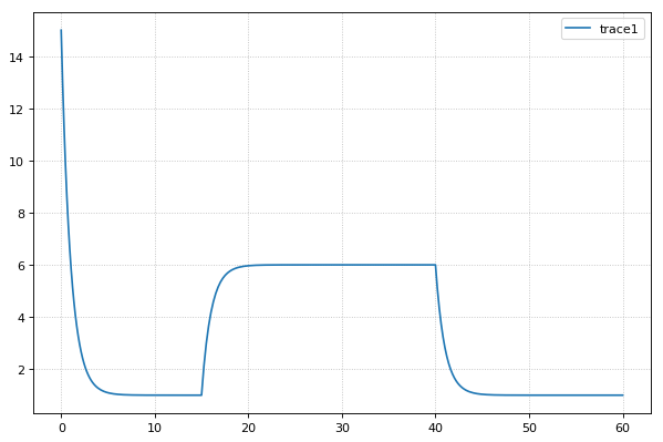
Merge multiple simulations

Example of merging multiple simulations. In between simulations a parameter is changed.

import tellurium as te
import numpy

r = te.loada ('''
    # Model Definition
    v1: $Xo -> S1;  k1*Xo;
    v2: S1 -> $w;   k2*S1;

    # Initialize constants
    k1 = 1; k2 = 1; S1 = 15; Xo = 1;
''')

# Time course simulation
m1 = r.simulate (0, 15, 100, ["Time","S1"]);
r.k1 = r.k1 * 6;
m2 = r.simulate (15, 40, 100, ["Time","S1"]);
r.k1 = r.k1 / 6;
m3 = r.simulate (40, 60, 100, ["Time","S1"]);

m = numpy.vstack([m1, m2, m3])
p = te.plot(m[:,0], m[:,1], name='trace1')

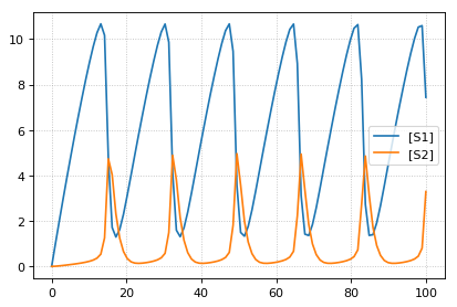
Relaxation oscillator

Oscillator that uses positive and negative feedback. An example of a relaxation oscillator.

import tellurium as te

r = te.loada ('''
  v1: $Xo -> S1; k1*Xo;
  v2:  S1 -> S2; k2*S1*S2^h/(10 + S2^h) + k3*S1;
  v3:  S2 -> $w; k4*S2;

  # Initialize
  h  = 2; # Hill coefficient
  k1 = 1; k2 = 2; Xo = 1;
  k3 = 0.02; k4 = 1;
''')

result = r.simulate(0, 100, 100)
r.plot(result);

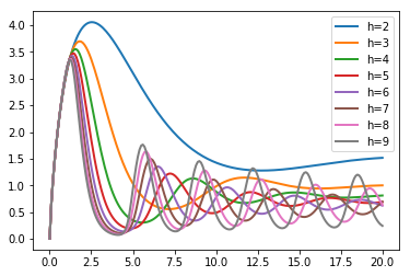
Scan hill coefficient

Negative Feedback model where we scan over the value of the Hill coefficient.

import tellurium as te
import numpy as np

r = te.loada ('''
  // Reactions:
  J0: $X0 => S1; (J0_VM1*(X0 - S1/J0_Keq1))/(1 + X0 + S1 + S4^J0_h);
  J1: S1 => S2; (10*S1 - 2*S2)/(1 + S1 + S2);
  J2: S2 => S3; (10*S2 - 2*S3)/(1 + S2 + S3);
  J3: S3 => S4; (10*S3 - 2*S4)/(1 + S3 + S4);
  J4: S4 => $X1; (J4_V4*S4)/(J4_KS4 + S4);

  // Species initializations:
  S1 = 0;
  S2 = 0;
  S3 = 0;
  S4 = 0;
  X0 = 10;
  X1 = 0;

  // Variable initializations:
  J0_VM1 = 10;
  J0_Keq1 = 10;
  J0_h = 2;
  J4_V4 = 2.5;
  J4_KS4 = 0.5;

  // Other declarations:
  const J0_VM1, J0_Keq1, J0_h, J4_V4, J4_KS4;
''')

# time vector
result = r.simulate (0, 20, 201, ['time'])

h_values = [r.J0_h + k for k in range(0,8)]
for h in h_values:
    r.reset()
    r.J0_h = h
    m = r.simulate(0, 20, 201, ['S1'])
    result = np.hstack([result, m])

te.plotArray(result, labels=['h={}'.format(int(h)) for h in h_values])
pass

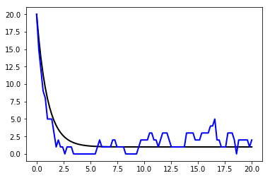
Compare simulations

import tellurium as te

r = te.loada ('''
     v1: $Xo -> S1;  k1*Xo;
     v2: S1 -> $w;   k2*S1;

     //initialize.  Deterministic process.
     k1 = 1; k2 = 1; S1 = 20; Xo = 1;
''')

m1 = r.simulate (0,20,100);

# Stochastic process
r.resetToOrigin()
r.setSeed(1234)
m2 = r.gillespie(0, 20, 100, ['time', 'S1'])

# plot all the results together
te.plotArray(m1, color="black", show=False)
te.plotArray(m2, color="blue");

Sinus injection

Example that show how to inject a sinusoidal into the model and use events to switch it off and on.

import tellurium as te
import numpy

r = te.loada ('''
    # Inject sin wave into model
    Xo := sin (time*0.5)*switch + 2;

    # Model Definition
    v1: $Xo -> S1;  k1*Xo;
    v2: S1 -> S2;   k2*S1;
    v3: S2 -> $X1;  k3*S2;

    at (time > 40): switch = 1;
    at (time > 80): switch = 0.5;

    # Initialize constants
    k1 = 1; k2 = 1; k3 = 3; S1 = 3;
    S2 = 0;
    switch = 0;
''')

result = r.simulate (0, 100, 200, ['time', 'S1', 'S2'])
r.plot(result);

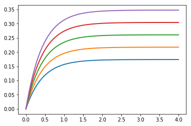
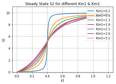
Protein phosphorylation cycle

Simple protein phosphorylation cycle. Steady state concentation of the phosphorylated protein is plotted as a function of the cycle kinase. In addition, the plot is repeated for various values of Km.

import tellurium as te
import numpy as np
import matplotlib.pyplot as plt

r = te.loada ('''
   S1 -> S2; k1*S1/(Km1 + S1);
   S2 -> S1; k2*S2/(Km2 + S2);

   k1 = 0.1; k2 = 0.4; S1 = 10; S2 = 0;
   Km1 = 0.1; Km2 = 0.1;
''')

r.conservedMoietyAnalysis = True

for i in range (1,8):
  numbers = np.linspace (0, 1.2, 200)
  result = np.empty ([0,2])
  for value in numbers:
      r.k1 = value
      r.steadyState()
      row = np.array ([value, r.S2])
      result = np.vstack ((result, row))
  te.plotArray(result, show=False, labels=['Km1={}'.format(r.Km1)],
               resetColorCycle=False,
               xlabel='k1', ylabel="S2",
               title="Steady State S2 for different Km1 & Km2",
               ylim=[-0.1, 11], grid=True)
  r.k1 = 0.1
  r.Km1 = r.Km1 + 0.5;
  r.Km2 = r.Km2 + 0.5;
plt.show()

Miscellaneous

How to install additional packages

If you are using Tellurium notebook or Tellurium Spyder, you can install additional package using installPackage function. In Tellurium Spyder, you can also install packages using included command Prompt. For more information, see Running Command Prompt for Tellurium Spyder.

import tellurium as te
# install cobra (https://github.com/opencobra/cobrapy)
te.installPackage('cobra')
# update cobra to latest version
te.upgradePackage('cobra')
# remove cobra
# te.removePackage('cobra')