Tellurium Methods¶

Installing Packages¶

Tellurium provides utility methods for installing Python packages from PyPI. These methods simply delegate to pip, and are usually more reliable than running !pip install xyz.

tellurium.installPackage(name)[source]¶

Install pip package. This has the advantage you don’t have to manually track down the currently running Python interpreter and switch to the command line (useful e.g. in the Tellurium notebook viewer).

Parameters:	name – package name
Returns:

tellurium.upgradePackage(name)[source]¶

Upgrade pip package.

Parameters:	name – package name
Returns:

tellurium.searchPackage(name)[source]¶

Search pip package for package name.

Parameters:	name – package name
Returns:

import tellurium as te
# install cobra (https://github.com/opencobra/cobrapy)
te.installPackage('cobra')
# update cobra to latest version
te.upgradePackage('cobra')
# remove cobra
# te.removePackage('cobra')

Requirement already satisfied: cobra in /home/poltergeist/.config/Tellurium/telocal/python-3.6.1/lib/python3.6/site-packages
Requirement already satisfied: numpy>=1.6 in /home/poltergeist/.config/Tellurium/telocal/python-3.6.1/lib/python3.6/site-packages (from cobra)
Requirement already satisfied: tabulate in /home/poltergeist/.config/Tellurium/telocal/python-3.6.1/lib/python3.6/site-packages (from cobra)
Requirement already satisfied: future in /home/poltergeist/.config/Tellurium/telocal/python-3.6.1/lib/python3.6/site-packages (from cobra)
Requirement already satisfied: swiglpk in /home/poltergeist/.config/Tellurium/telocal/python-3.6.1/lib/python3.6/site-packages (from cobra)
Requirement already satisfied: pandas>=0.17.0 in /home/poltergeist/.config/Tellurium/telocal/python-3.6.1/lib/python3.6/site-packages (from cobra)
Requirement already satisfied: optlang>=1.2.1 in /home/poltergeist/.config/Tellurium/telocal/python-3.6.1/lib/python3.6/site-packages (from cobra)
Requirement already satisfied: ruamel.yaml<0.15 in /home/poltergeist/.config/Tellurium/telocal/python-3.6.1/lib/python3.6/site-packages (from cobra)
Requirement already satisfied: pytz>=2011k in /home/poltergeist/.config/Tellurium/telocal/python-3.6.1/lib/python3.6/site-packages (from pandas>=0.17.0->cobra)
Requirement already satisfied: python-dateutil>=2 in /home/poltergeist/.config/Tellurium/telocal/python-3.6.1/lib/python3.6/site-packages (from pandas>=0.17.0->cobra)
Requirement already satisfied: sympy>=1.0.0 in /home/poltergeist/.config/Tellurium/telocal/python-3.6.1/lib/python3.6/site-packages (from optlang>=1.2.1->cobra)
Requirement already satisfied: six>=1.9.0 in /home/poltergeist/.config/Tellurium/telocal/python-3.6.1/lib/python3.6/site-packages (from optlang>=1.2.1->cobra)
Requirement already satisfied: mpmath>=0.19 in /home/poltergeist/.config/Tellurium/telocal/python-3.6.1/lib/python3.6/site-packages (from sympy>=1.0.0->optlang>=1.2.1->cobra)
Requirement already up-to-date: cobra in /home/poltergeist/.config/Tellurium/telocal/python-3.6.1/lib/python3.6/site-packages
Requirement already up-to-date: numpy>=1.6 in /home/poltergeist/.config/Tellurium/telocal/python-3.6.1/lib/python3.6/site-packages (from cobra)
Requirement already up-to-date: tabulate in /home/poltergeist/.config/Tellurium/telocal/python-3.6.1/lib/python3.6/site-packages (from cobra)
Requirement already up-to-date: future in /home/poltergeist/.config/Tellurium/telocal/python-3.6.1/lib/python3.6/site-packages (from cobra)
Requirement already up-to-date: swiglpk in /home/poltergeist/.config/Tellurium/telocal/python-3.6.1/lib/python3.6/site-packages (from cobra)
Requirement already up-to-date: pandas>=0.17.0 in /home/poltergeist/.config/Tellurium/telocal/python-3.6.1/lib/python3.6/site-packages (from cobra)
Requirement already up-to-date: optlang>=1.2.1 in /home/poltergeist/.config/Tellurium/telocal/python-3.6.1/lib/python3.6/site-packages (from cobra)
Requirement already up-to-date: ruamel.yaml<0.15 in /home/poltergeist/.config/Tellurium/telocal/python-3.6.1/lib/python3.6/site-packages (from cobra)
Requirement already up-to-date: pytz>=2011k in /home/poltergeist/.config/Tellurium/telocal/python-3.6.1/lib/python3.6/site-packages (from pandas>=0.17.0->cobra)
Requirement already up-to-date: python-dateutil>=2 in /home/poltergeist/.config/Tellurium/telocal/python-3.6.1/lib/python3.6/site-packages (from pandas>=0.17.0->cobra)
Requirement already up-to-date: sympy>=1.0.0 in /home/poltergeist/.config/Tellurium/telocal/python-3.6.1/lib/python3.6/site-packages (from optlang>=1.2.1->cobra)
Requirement already up-to-date: six>=1.9.0 in /home/poltergeist/.config/Tellurium/telocal/python-3.6.1/lib/python3.6/site-packages (from optlang>=1.2.1->cobra)
Requirement already up-to-date: mpmath>=0.19 in /home/poltergeist/.config/Tellurium/telocal/python-3.6.1/lib/python3.6/site-packages (from sympy>=1.0.0->optlang>=1.2.1->cobra)

Utility Methods¶

The most useful methods here are the notices routines. Roadrunner will offen issue warning or informational messages. For repeated simulation such messages will clutter up the outputs. noticesOff and noticesOn can be used to turn on an off the messages.

tellurium.getVersionInfo()[source]¶

Returns version information for tellurium included packages.

Returns:	list of tuples (package, version)

tellurium.printVersionInfo()[source]¶

Prints version information for tellurium included packages.

Version information¶

Tellurium’s version can be obtained via te.__version__. .printVersionInfo() also returns information from certain constituent packages.

import tellurium as te

# to get the tellurium version use
print('te.__version__')
print(te.__version__)
# or
print('te.getTelluriumVersion()')
print(te.getTelluriumVersion())

# to print the full version info use
print('-' * 80)
te.printVersionInfo()
print('-' * 80)

/home/poltergeist/.config/Tellurium/telocal/python-3.6.1/lib/python3.6/site-packages/matplotlib/__init__.py:1405: UserWarning:
This call to matplotlib.use() has no effect because the backend has already
been chosen; matplotlib.use() must be called before pylab, matplotlib.pyplot,
or matplotlib.backends is imported for the first time.

  warnings.warn(_use_error_msg)

te.__version__
2.0.1
te.getTelluriumVersion()
2.0.1
--------------------------------------------------------------------------------
tellurium : 2.0.1
roadrunner : 1.4.21; Compiler: gcc 4.8.2, C++ version: 199711; JIT Compiler: LLVM-3.3; Date: Jul  5 2017, 18:38:02; LibSBML Version: 5.14.0
antimony : 2.9.3
libsbml : 5.15.0
libsedml : 402
phrasedml : 1.0.7
--------------------------------------------------------------------------------

Repeat simulation without notification¶

from builtins import range
# Load SBML file
r = te.loada("""
model test
    J0: X0 -> X1; k1*X0;
    X0 = 10; X1=0;
    k1 = 0.2
end
""")

import matplotlib.pyplot as plt

# Turn of notices so they don't clutter the output
te.noticesOff()
for i in range(0, 20):
    result = r.simulate (0, 10)
    r.reset()
    r.plot(result, loc=None, show=False,
           linewidth=2.0, linestyle='-', color='black', alpha=0.8)
    r.k1 = r.k1 + 0.2
# Turn the notices back on
te.noticesOn()

File helpers for reading and writing¶

# create tmp file
import tempfile
ftmp = tempfile.NamedTemporaryFile(suffix=".xml")
# load model
r = te.loada('S1 -> S2; k1*S1; k1 = 0.1; S1 = 10')
# save to file
te.saveToFile(ftmp.name, r.getMatlab())

# or easier via
r.exportToMatlab(ftmp.name)

# load file
sbmlstr = te.readFromFile(ftmp.name)
print('%' + '*'*80)
print('Converted MATLAB code')
print('%' + '*'*80)
print(sbmlstr)

%********************************************************************************
Converted MATLAB code
%********************************************************************************
%  How to use:
%
%  __main takes 3 inputs and returns 3 outputs.
%
%  [t x rInfo] = __main(tspan,solver,options)
%  INPUTS:
%  tspan - the time vector for the simulation. It can contain every time point,
%  or just the start and end (e.g. [0 1 2 3] or [0 100]).
%  solver - the function handle for the odeN solver you wish to use (e.g. @ode23s).
%  options - this is the options structure returned from the MATLAB odeset
%  function used for setting tolerances and other parameters for the solver.
%
%  OUTPUTS:
%  t - the time vector that corresponds with the solution. If tspan only contains
%  the start and end times, t will contain points spaced out by the solver.
%  x - the simulation results.
%  rInfo - a structure containing information about the model. The fields
%  within rInfo are:
%     stoich - the stoichiometry matrix of the model
%     floatingSpecies - a cell array containing floating species name, initial
%     value, and indicator of the units being inconcentration or amount
%     compartments - a cell array containing compartment names and volumes
%     params - a cell array containing parameter names and values
%     boundarySpecies - a cell array containing boundary species name, initial
%     value, and indicator of the units being inconcentration or amount
%     rateRules - a cell array containing the names of variables used in a rate rule
%
%  Sample function call:
%     options = odeset('RelTol',1e-12,'AbsTol',1e-9);
%     [t x rInfo] = __main(linspace(0,100,100),@ode23s,options);
%
function [t x rInfo] = __main(tspan,solver,options)
    % initial conditions
    [x rInfo] = model();

    % initial assignments

    % assignment rules

    % run simulation
    [t x] = feval(solver,@model,tspan,x,options);

    % assignment rules

function [xdot rInfo] = model(time,x)
%  x(1)        S1
%  x(2)        S2

% List of Compartments
vol__default_compartment = 1;               %default_compartment

% Global Parameters
rInfo.g_p1 = 0.1;           % k1

if (nargin == 0)

    % set initial conditions
   xdot(1) = 10*vol__default_compartment;           % S1 = S1 [Concentration]
   xdot(2) = 0*vol__default_compartment;            % S2 = S2 [Concentration]

   % reaction info structure
   rInfo.stoich = [
      -1
      1
   ];

   rInfo.floatingSpecies = {                % Each row: [Species Name, Initial Value, isAmount (1 for amount, 0 for concentration)]
      'S1' , 10, 0
      'S2' , 0, 0
   };

   rInfo.compartments = {           % Each row: [Compartment Name, Value]
      'default_compartment' , 1
   };

   rInfo.params = {         % Each row: [Parameter Name, Value]
      'k1' , 0.1
   };

   rInfo.boundarySpecies = {                % Each row: [Species Name, Initial Value, isAmount (1 for amount, 0 for concentration)]
   };

   rInfo.rateRules = {               % List of variables involved in a rate rule
   };

else

    % calculate rates of change
   R0 = rInfo.g_p1*(x(1));

   xdot = [
      - R0
      + R0
   ];
end;


%listOfSupportedFunctions
function z = pow (x,y)
    z = x^y;


function z = sqr (x)
    z = x*x;


function z = piecewise(varargin)
            numArgs = nargin;
            result = 0;
            foundResult = 0;
            for k=1:2: numArgs-1
                    if varargin{k+1} == 1
                            result = varargin{k};
                            foundResult = 1;
                            break;
                    end
            end
            if foundResult == 0
                    result = varargin{numArgs};
            end
            z = result;


function z = gt(a,b)
   if a > b
      z = 1;
   else
      z = 0;
   end


function z = lt(a,b)
   if a < b
      z = 1;
   else
      z = 0;
   end


function z = geq(a,b)
   if a >= b
      z = 1;
   else
      z = 0;
   end


function z = leq(a,b)
   if a <= b
      z = 1;
   else
      z = 0;
   end


function z = neq(a,b)
   if a ~= b
      z = 1;
   else
      z = 0;
   end


function z = and(varargin)
            result = 1;
            for k=1:nargin
               if varargin{k} ~= 1
                  result = 0;
                  break;
               end
            end
            z = result;


function z = or(varargin)
            result = 0;
            for k=1:nargin
               if varargin{k} ~= 0
                  result = 1;
                  break;
               end
            end
            z = result;


function z = xor(varargin)
            foundZero = 0;
            foundOne = 0;
            for k = 1:nargin
                    if varargin{k} == 0
                       foundZero = 1;
                    else
                       foundOne = 1;
                    end
            end
            if foundZero && foundOne
                    z = 1;
            else
              z = 0;
            end



function z = not(a)
   if a == 1
      z = 0;
   else
      z = 1;
   end


function z = root(a,b)
    z = a^(1/b);

Model Loading¶

There are a variety of methods to load models into libRoadrunner.

tellurium.loada(ant)[source]¶

Load model from Antimony string.

Load Antimony¶

Antimony files can be read with te.loada or te.loadAntimonyModel. For SBML te.loadSBMLModel, for CellML te.loadCellMLModel is used. All the functions accept either model strings or respective model files.

import tellurium as te
te.setDefaultPlottingEngine('matplotlib')

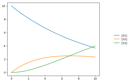
# Load an antimony model
ant_model = '''
    S1 -> S2; k1*S1;
    S2 -> S3; k2*S2;

    k1= 0.1; k2 = 0.2;
    S1 = 10; S2 = 0; S3 = 0;
'''
# At the most basic level one can load the SBML model directly using libRoadRunner
print('---  load using roadrunner ---')
import roadrunner
# convert to SBML model
sbml_model = te.antimonyToSBML(ant_model)
r = roadrunner.RoadRunner(sbml_model)
result = r.simulate(0, 10, 100)
r.plot(result)

# The method loada is simply a shortcut to loadAntimonyModel
print('---  load using tellurium ---')
r = te.loada(ant_model)
result = r.simulate (0, 10, 100)
r.plot(result)

# same like
r = te.loadAntimonyModel(ant_model)

---  load using roadrunner ---

---  load using tellurium ---

Interconversion Utilities¶

Use these routines interconvert verious standard formats

tellurium.antimonyToSBML(ant)[source]¶

Convert Antimony to SBML string.

Parameters:	ant (str \| file) – Antimony string or file
Returns:	SBML
Return type:	str

tellurium.antimonyToCellML(ant)[source]¶

Convert Antimony to CellML string.

Parameters:	ant (str \| file) – Antimony string or file
Returns:	CellML
Return type:	str

tellurium.sbmlToAntimony(sbml)[source]¶

Convert SBML to antimony string.

Parameters:	sbml (str \| file) – SBML string or file
Returns:	Antimony
Return type:	str

tellurium.sbmlToCellML(sbml)[source]¶

Convert SBML to CellML string.

Parameters:	sbml (str \| file) – SBML string or file
Returns:	CellML
Return type:	str

tellurium.cellmlToAntimony(cellml)[source]¶

Convert CellML to antimony string.

Parameters:	cellml (str \| file) – CellML string or file
Returns:	antimony
Return type:	str

tellurium.cellmlToSBML(cellml)[source]¶

Convert CellML to SBML string.

Parameters:	cellml (str \| file) – CellML string or file
Returns:	SBML
Return type:	str

Antimony, SBML, CellML¶

Tellurium can convert between Antimony, SBML, and CellML.

import tellurium as te

# antimony model
ant_model = """
    S1 -> S2; k1*S1;
    S2 -> S3; k2*S2;

    k1= 0.1; k2 = 0.2;
    S1 = 10; S2 = 0; S3 = 0;
"""

# convert to SBML
sbml_model = te.antimonyToSBML(ant_model)
print('sbml_model')
print('*'*80)
# print first 10 lines
for line in list(sbml_model.splitlines())[:10]:
    print(line)
print('...')

# convert to CellML
cellml_model = te.antimonyToCellML(ant_model)
print('cellml_model (from Antimony)')
print('*'*80)
# print first 10 lines
for line in list(cellml_model.splitlines())[:10]:
    print(line)
print('...')

# or from the sbml
cellml_model = te.sbmlToCellML(sbml_model)
print('cellml_model (from SBML)')
print('*'*80)
# print first 10 lines
for line in list(cellml_model.splitlines())[:10]:
    print(line)
print('...')

sbml_model
****************************************************************************
<?xml version="1.0" encoding="UTF-8"?>
<!-- Created by libAntimony version v2.9.3 with libSBML version 5.15.0. -->
<sbml xmlns="http://www.sbml.org/sbml/level3/version1/core" level="3" version="1">
  <model id="__main" name="__main">
    <listOfCompartments>
      <compartment sboTerm="SBO:0000410" id="default_compartment" spatialDimensions="3" size="1" constant="true"/>
    </listOfCompartments>
    <listOfSpecies>
      <species id="S1" compartment="default_compartment" initialConcentration="10" hasOnlySubstanceUnits="false" boundaryCondition="false" constant="false"/>
      <species id="S2" compartment="default_compartment" initialConcentration="0" hasOnlySubstanceUnits="false" boundaryCondition="false" constant="false"/>
...
cellml_model (from Antimony)
****************************************************************************
<?xml version="1.0"?>
<model xmlns:cellml="http://www.cellml.org/cellml/1.1#" xmlns="http://www.cellml.org/cellml/1.1#" name="__main">
<component name="__main">
<variable initial_value="10" name="S1" units="dimensionless"/>
<variable initial_value="0" name="S2" units="dimensionless"/>
<variable initial_value="0.1" name="k1" units="dimensionless"/>
<variable name="_J0" units="dimensionless"/>
<variable initial_value="0" name="S3" units="dimensionless"/>
<variable initial_value="0.2" name="k2" units="dimensionless"/>
<variable name="_J1" units="dimensionless"/>
...
cellml_model (from SBML)
****************************************************************************
<?xml version="1.0"?>
<model xmlns:cellml="http://www.cellml.org/cellml/1.1#" xmlns="http://www.cellml.org/cellml/1.1#" name="__main">
<component name="__main">
<variable initial_value="10" name="S1" units="dimensionless"/>
<variable initial_value="0" name="S2" units="dimensionless"/>
<variable initial_value="0" name="S3" units="dimensionless"/>
<variable initial_value="0.1" name="k1" units="dimensionless"/>
<variable initial_value="0.2" name="k2" units="dimensionless"/>
<variable name="_J0" units="dimensionless"/>
<variable name="_J1" units="dimensionless"/>
...

Export Utilities¶

Use these routines to convert the current model state into other formats, like Matlab, CellML, Antimony and SBML.

class tellurium.tellurium.ExtendedRoadRunner(*args, **kwargs)[source]¶

exportToAntimony(filePath, current=True)[source]¶

Save current model as Antimony file.

Parameters:	current (bool) – export current model state filePath (str) – file path of Antimony file

exportToCellML(filePath, current=True)[source]¶

Save current model as CellML file.

Parameters:	current (bool) – export current model state filePath (str) – file path of CellML file

exportToMatlab(filePath, current=True)[source]¶

Save current model as Matlab file. To save the original model loaded into roadrunner use current=False.

Parameters:	self (RoadRunner.roadrunner) – RoadRunner instance filePath (str) – file path of Matlab file

exportToSBML(filePath, current=True)[source]¶

Save current model as SBML file.

Parameters:	current (bool) – export current model state filePath (str) – file path of SBML file

getAntimony(current=False)[source]¶

Antimony string of the original model loaded into roadrunner.

Parameters:	current (bool) – return current model state
Returns:	Antimony
Return type:	str

getCellML(current=False)[source]¶

CellML string of the original model loaded into roadrunner.

Parameters:	current (bool) – return current model state
Returns:	CellML string
Return type:	str

getCurrentAntimony()[source]¶

Antimony string of the current model state.

See also: getAntimony() :return: Antimony :rtype: str

getCurrentCellML()[source]¶

CellML string of current model state.

See also: getCellML() :returns: CellML string :rtype: str

getCurrentMatlab()[source]¶

Matlab string of current model state.

Parameters:	current (bool) – return current model state
Returns:	Matlab string
Return type:	str

getMatlab(current=False)[source]¶

Matlab string of the original model loaded into roadrunner.

See also: getCurrentMatlab() :returns: Matlab string :rtype: str

SBML¶

Given a RoadRunner instance, you can get an SBML representation of the current state of the model using getCurrentSBML. You can also get the initial SBML from when the model was loaded using getSBML. Finally, exportToSBML can be used to export the current model state to a file.

import tellurium as te
te.setDefaultPlottingEngine('matplotlib')
import tempfile

# load model
r = te.loada('S1 -> S2; k1*S1; k1 = 0.1; S1 = 10')
# file for export
f_sbml = tempfile.NamedTemporaryFile(suffix=".xml")

# export current model state
r.exportToSBML(f_sbml.name)

# to export the initial state when the model was loaded
# set the current argument to False
r.exportToSBML(f_sbml.name, current=False)

# The string representations of the current model are available via
str_sbml = r.getCurrentSBML()

# and of the initial state when the model was loaded via
str_sbml = r.getSBML()
print(str_sbml)

<?xml version="1.0" encoding="UTF-8"?>
<!-- Created by libAntimony version v2.9.3 with libSBML version 5.15.0. -->
<sbml xmlns="http://www.sbml.org/sbml/level3/version1/core" level="3" version="1">
  <model id="__main" name="__main">
    <listOfCompartments>
      <compartment sboTerm="SBO:0000410" id="default_compartment" spatialDimensions="3" size="1" constant="true"/>
    </listOfCompartments>
    <listOfSpecies>
      <species id="S1" compartment="default_compartment" initialConcentration="10" hasOnlySubstanceUnits="false" boundaryCondition="false" constant="false"/>
      <species id="S2" compartment="default_compartment" hasOnlySubstanceUnits="false" boundaryCondition="false" constant="false"/>
    </listOfSpecies>
    <listOfParameters>
      <parameter id="k1" value="0.1" constant="true"/>
    </listOfParameters>
    <listOfReactions>
      <reaction id="_J0" reversible="true" fast="false">
        <listOfReactants>
          <speciesReference species="S1" stoichiometry="1" constant="true"/>
        </listOfReactants>
        <listOfProducts>
          <speciesReference species="S2" stoichiometry="1" constant="true"/>
        </listOfProducts>
        <kineticLaw>
          <math xmlns="http://www.w3.org/1998/Math/MathML">
            <apply>
              <times/>
              <ci> k1 </ci>
              <ci> S1 </ci>
            </apply>
          </math>
        </kineticLaw>
      </reaction>
    </listOfReactions>
  </model>
</sbml>

Antimony¶

Similar to the SBML functions above, you can also use the functions getCurrentAntimony and exportToAntimony to get or export the current Antimony representation.

import tellurium as te
import tempfile

# load model
r = te.loada('S1 -> S2; k1*S1; k1 = 0.1; S1 = 10')
# file for export
f_antimony = tempfile.NamedTemporaryFile(suffix=".txt")

# export current model state
r.exportToAntimony(f_antimony.name)

# to export the initial state when the model was loaded
# set the current argument to False
r.exportToAntimony(f_antimony.name, current=False)

# The string representations of the current model are available via
str_antimony = r.getCurrentAntimony()

# and of the initial state when the model was loaded via
str_antimony = r.getAntimony()
print(str_antimony)

// Created by libAntimony v2.9.3
// Compartments and Species:
species S1, S2;

// Reactions:
_J0: S1 -> S2; k1*S1;

// Species initializations:
S1 = 10;
S2 = ;

// Variable initializations:
k1 = 0.1;

// Other declarations:
const k1;

CellML¶

Tellurium also has functions for exporting the current model state to CellML. These functionalities rely on using Antimony to perform the conversion.

import tellurium as te
import tempfile

# load model
r = te.loada('S1 -> S2; k1*S1; k1 = 0.1; S1 = 10')
# file for export
f_cellml = tempfile.NamedTemporaryFile(suffix=".cellml")

# export current model state
r.exportToCellML(f_cellml.name)

# to export the initial state when the model was loaded
# set the current argument to False
r.exportToCellML(f_cellml.name, current=False)

# The string representations of the current model are available via
str_cellml = r.getCurrentCellML()

# and of the initial state when the model was loaded via
str_cellml = r.getCellML()
print(str_cellml)

<?xml version="1.0"?>
<model xmlns:cellml="http://www.cellml.org/cellml/1.1#" xmlns="http://www.cellml.org/cellml/1.1#" name="__main">
<component name="__main">
<variable initial_value="10" name="S1" units="dimensionless"/>
<variable name="S2" units="dimensionless"/>
<variable initial_value="0.1" name="k1" units="dimensionless"/>
<variable name="_J0" units="dimensionless"/>
<math xmlns="http://www.w3.org/1998/Math/MathML">
<apply>
<eq/>
<ci>_J0</ci>
<apply>
<times/>
<ci>k1</ci>
<ci>S1</ci>
</apply>
</apply>
</math>
<variable name="time" units="dimensionless"/>
<math xmlns="http://www.w3.org/1998/Math/MathML">
<apply>
<eq/>
<apply>
<diff/>
<bvar>
<ci>time</ci>
</bvar>
<ci>S2</ci>
</apply>
<ci>_J0</ci>
</apply>
</math>
<math xmlns="http://www.w3.org/1998/Math/MathML">
<apply>
<eq/>
<apply>
<diff/>
<bvar>
<ci>time</ci>
</bvar>
<ci>S1</ci>
</apply>
<apply>
<minus/>
<ci>_J0</ci>
</apply>
</apply>
</math>
</component>
<group>
<relationship_ref relationship="encapsulation"/>
<component_ref component="__main"/>
</group>
</model>

Matlab¶

To export the current model state to MATLAB, use getCurrentMatlab.

import tellurium as te
import tempfile

# load model
r = te.loada('S1 -> S2; k1*S1; k1 = 0.1; S1 = 10')
# file for export
f_matlab = tempfile.NamedTemporaryFile(suffix=".m")

# export current model state
r.exportToMatlab(f_matlab.name)

# to export the initial state when the model was loaded
# set the current argument to False
r.exportToMatlab(f_matlab.name, current=False)

# The string representations of the current model are available via
str_matlab = r.getCurrentMatlab()

# and of the initial state when the model was loaded via
str_matlab = r.getMatlab()
print(str_matlab)

%  How to use:
%
%  __main takes 3 inputs and returns 3 outputs.
%
%  [t x rInfo] = __main(tspan,solver,options)
%  INPUTS:
%  tspan - the time vector for the simulation. It can contain every time point,
%  or just the start and end (e.g. [0 1 2 3] or [0 100]).
%  solver - the function handle for the odeN solver you wish to use (e.g. @ode23s).
%  options - this is the options structure returned from the MATLAB odeset
%  function used for setting tolerances and other parameters for the solver.
%
%  OUTPUTS:
%  t - the time vector that corresponds with the solution. If tspan only contains
%  the start and end times, t will contain points spaced out by the solver.
%  x - the simulation results.
%  rInfo - a structure containing information about the model. The fields
%  within rInfo are:
%     stoich - the stoichiometry matrix of the model
%     floatingSpecies - a cell array containing floating species name, initial
%     value, and indicator of the units being inconcentration or amount
%     compartments - a cell array containing compartment names and volumes
%     params - a cell array containing parameter names and values
%     boundarySpecies - a cell array containing boundary species name, initial
%     value, and indicator of the units being inconcentration or amount
%     rateRules - a cell array containing the names of variables used in a rate rule
%
%  Sample function call:
%     options = odeset('RelTol',1e-12,'AbsTol',1e-9);
%     [t x rInfo] = __main(linspace(0,100,100),@ode23s,options);
%
function [t x rInfo] = __main(tspan,solver,options)
    % initial conditions
    [x rInfo] = model();

    % initial assignments

    % assignment rules

    % run simulation
    [t x] = feval(solver,@model,tspan,x,options);

    % assignment rules

function [xdot rInfo] = model(time,x)
%  x(1)        S1
%  x(2)        S2

% List of Compartments
vol__default_compartment = 1;               %default_compartment

% Global Parameters
rInfo.g_p1 = 0.1;           % k1

if (nargin == 0)

    % set initial conditions
   xdot(1) = 10*vol__default_compartment;           % S1 = S1 [Concentration]
   xdot(2) = 0*vol__default_compartment;            % S2 = S2 [Concentration]

   % reaction info structure
   rInfo.stoich = [
      -1
      1
   ];

   rInfo.floatingSpecies = {                % Each row: [Species Name, Initial Value, isAmount (1 for amount, 0 for concentration)]
      'S1' , 10, 0
      'S2' , 0, 0
   };

   rInfo.compartments = {           % Each row: [Compartment Name, Value]
      'default_compartment' , 1
   };

   rInfo.params = {         % Each row: [Parameter Name, Value]
      'k1' , 0.1
   };

   rInfo.boundarySpecies = {                % Each row: [Species Name, Initial Value, isAmount (1 for amount, 0 for concentration)]
   };

   rInfo.rateRules = {               % List of variables involved in a rate rule
   };

else

    % calculate rates of change
   R0 = rInfo.g_p1*(x(1));

   xdot = [
      - R0
      + R0
   ];
end;


%listOfSupportedFunctions
function z = pow (x,y)
    z = x^y;


function z = sqr (x)
    z = x*x;


function z = piecewise(varargin)
            numArgs = nargin;
            result = 0;
            foundResult = 0;
            for k=1:2: numArgs-1
                    if varargin{k+1} == 1
                            result = varargin{k};
                            foundResult = 1;
                            break;
                    end
            end
            if foundResult == 0
                    result = varargin{numArgs};
            end
            z = result;


function z = gt(a,b)
   if a > b
      z = 1;
   else
      z = 0;
   end


function z = lt(a,b)
   if a < b
      z = 1;
   else
      z = 0;
   end


function z = geq(a,b)
   if a >= b
      z = 1;
   else
      z = 0;
   end


function z = leq(a,b)
   if a <= b
      z = 1;
   else
      z = 0;
   end


function z = neq(a,b)
   if a ~= b
      z = 1;
   else
      z = 0;
   end


function z = and(varargin)
            result = 1;
            for k=1:nargin
               if varargin{k} ~= 1
                  result = 0;
                  break;
               end
            end
            z = result;


function z = or(varargin)
            result = 0;
            for k=1:nargin
               if varargin{k} ~= 0
                  result = 1;
                  break;
               end
            end
            z = result;


function z = xor(varargin)
            foundZero = 0;
            foundOne = 0;
            for k = 1:nargin
                    if varargin{k} == 0
                       foundZero = 1;
                    else
                       foundOne = 1;
                    end
            end
            if foundZero && foundOne
                    z = 1;
            else
              z = 0;
            end



function z = not(a)
   if a == 1
      z = 0;
   else
      z = 1;
   end


function z = root(a,b)
    z = a^(1/b);

Using Antimony Directly¶

The above examples rely on Antimony as in intermediary between formats. You can use this functionality directly using e.g. antimony.getCellMLString. A comprehensive set of functions can be found in the Antimony API documentation.

import antimony
antimony.loadAntimonyString('''S1 -> S2; k1*S1; k1 = 0.1; S1 = 10''')
ant_str = antimony.getCellMLString(antimony.getMainModuleName())
print(ant_str)

<?xml version="1.0"?>
<model xmlns:cellml="http://www.cellml.org/cellml/1.1#" xmlns="http://www.cellml.org/cellml/1.1#" name="__main">
<component name="__main">
<variable initial_value="10" name="S1" units="dimensionless"/>
<variable name="S2" units="dimensionless"/>
<variable initial_value="0.1" name="k1" units="dimensionless"/>
<variable name="_J0" units="dimensionless"/>
<math xmlns="http://www.w3.org/1998/Math/MathML">
<apply>
<eq/>
<ci>_J0</ci>
<apply>
<times/>
<ci>k1</ci>
<ci>S1</ci>
</apply>
</apply>
</math>
<variable name="time" units="dimensionless"/>
<math xmlns="http://www.w3.org/1998/Math/MathML">
<apply>
<eq/>
<apply>
<diff/>
<bvar>
<ci>time</ci>
</bvar>
<ci>S1</ci>
</apply>
<apply>
<minus/>
<ci>_J0</ci>
</apply>
</apply>
</math>
<math xmlns="http://www.w3.org/1998/Math/MathML">
<apply>
<eq/>
<apply>
<diff/>
<bvar>
<ci>time</ci>
</bvar>
<ci>S2</ci>
</apply>
<ci>_J0</ci>
</apply>
</math>
</component>
<group>
<relationship_ref relationship="encapsulation"/>
<component_ref component="__main"/>
</group>
</model>

Stochastic Simulation¶

Use these routines to carry out Gillespie style stochastic simulations.

class tellurium.tellurium.ExtendedRoadRunner(*args, **kwargs)[source]

getSeed(integratorName='gillespie')[source]¶

Current seed used by the integrator with integratorName. Defaults to the seed of the gillespie integrator.

Parameters:	integratorName (str) – name of the integrator for which the seed should be retured
Returns:	current seed
Return type:	float

gillespie(*args, **kwargs)[source]¶

Run a Gillespie stochastic simulation.

Sets the integrator to gillespie and performs simulation.

rr = te.loada ('S1 -> S2; k1*S1; k1 = 0.1; S1 = 40')
# Simulate from time zero to 40 time units
result = rr.gillespie (0, 40)
# Simulate on a grid with 10 points from start 0 to end time 40
rr.reset()
result = rr.gillespie (0, 40, 10)
# Simulate from time zero to 40 time units using the given selection list
# This means that the first column will be time and the second column species S1
rr.reset()
result = rr.gillespie (0, 40, selections=['time', 'S1'])
# Simulate from time zero to 40 time units, on a grid with 20 points
# using the give selection list
rr.reset()
result = rr.gillespie (0, 40, 20, ['time', 'S1'])
rr.plot(result)

Parameters:	seed (int) – seed for gillespie args – parameters for simulate kwargs – parameters for simulate
Returns:	simulation results

setSeed(seed, integratorName='gillespie')[source]¶

Set seed in integrator with integratorName. Defaults to the seed of the gillespie integrator.

Raises Error if integrator does not have key ‘seed’.

Parameters:	seed – seed to set integratorName (str) – name of the integrator for which the seed should be retured

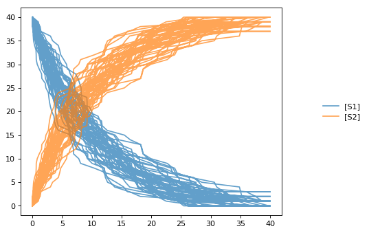
Stochastic simulation¶

Stochastic simulations can be run by changing the current integrator type to ‘gillespie’ or by using the r.gillespie function.

import tellurium as te
te.setDefaultPlottingEngine('matplotlib')
import numpy as np

r = te.loada('S1 -> S2; k1*S1; k1 = 0.1; S1 = 40')
r.integrator = 'gillespie'
r.integrator.seed = 1234

results = []
for k in range(1, 50):
    r.reset()
    s = r.simulate(0, 40)
    results.append(s)
    r.plot(s, show=False, alpha=0.7)
te.show()

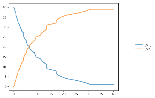
Seed¶

Setting the identical seed for all repeats results in identical traces in each simulation.

results = []
for k in range(1, 20):
    r.reset()
    r.setSeed(123456)
    s = r.simulate(0, 40)
    results.append(s)
    r.plot(s, show=False, loc=None, color='black', alpha=0.7)
te.show()

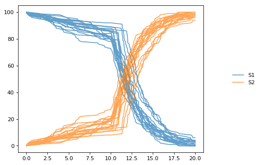
Combining Simulations¶

You can combine two timecourse simulations and change e.g. parameter values in between each simulation. The gillespie method simulates up to the given end time 10, after which you can make arbitrary changes to the model, then simulate again.

When using the te.plot function, you can pass the parameter names, which controls the names that will be used in the figure legend, and tags, which ensures that traces with the same tag will be drawn with the same color.

import tellurium as te
import numpy as np

r = te.loada('S1 -> S2; k1*S1; k1 = 0.02; S1 = 100')
r.setSeed(1234)
for k in range(1, 20):
    r.resetToOrigin()
    res1 = r.gillespie(0, 10)
    # change in parameter after the first half of the simulation
    r.k1 = r.k1*20
    res2 = r.gillespie (10, 20)
    sim = np.vstack([res1, res2])
    te.plot(sim[:,0], sim[:,1:], alpha=0.7, names=['S1', 'S2'], tags=['S1', 'S2'], show=False)
te.show()

Distributed Stochastic Simulation¶

Use these in order to run simulations in distributed environment.

class tellurium.StochasticSimulationModel(model=None, integrator='gillespie', seed=1234, variable_step_size=False, from_time=0, to_time=40, step_points=50)[source]¶

Distributed Stochastic Simulation Utility¶

Use these in order to run simulations in distributed environment. It uses the object defined with StochasticSimulationModel.

tellurium.distributed_stochastic_simulation(sc, stochastic_model_object, num_simulations, model_type='antimony')[source]¶

Plot Distributed Stochastic Simulation Results¶

To plot the results retrieved from distributed_stochastic_simulation.

tellurium.plot_stochastic_result(result)[source]¶

Distributed Parameter Scanning¶

Parameter Scanning one/more models in a distributed environment

tellurium.distributed_parameter_scanning(sc, list_of_models, function_name, antimony='antimony')[source]¶

Plotting Image of Parameter Scan¶

Helps in plotting the results parameter Scanning of one/more models run in a distributed environment

tellurium.plotImage(img)[source]¶

Distributed Sensitivity Analysis¶

Use these in order to run Sensitivity Analysis in distributed environment.

class tellurium.SensitivityAnalysis(model=None, sbml=False, conservedMoietyAnalysis=True)[source]¶

Distributed Sensitivity Analysis Utility¶

Running the Sensitivity analysis using the model created using tellurium.SensitivityAnalysis

tellurium.distributed_sensitivity_analysis(sc, senitivity_analysis_model, calculation=None)[source]¶

Math¶

Only one routine is currently available in this group which is a routine to compute the eigenvalues of given a matrix.

tellurium.getEigenvalues(m)[source]¶

Eigenvalues of matrix.

Convenience method for computing the eigenvalues of a matrix m Uses numpy eig to compute the eigenvalues.

Parameters:	m – numpy array
Returns:	numpy array containing eigenvalues

Plotting¶

Two useful plotting routines. They assume that the first column in the array is the x-axis and the second and subsequent columns represent curves on the y-axis.

tellurium.plotArray(result, loc='upper right', show=True, resetColorCycle=True, xlabel=None, ylabel=None, title=None, xlim=None, ylim=None, xscale='linear', yscale='linear', grid=False, labels=None, **kwargs)[source]¶

Plot an array.

The first column of the array must be the x-axis and remaining columns the y-axis. Returns a handle to the plotting object. Note that you can add plotting options as named key values after the array. To add a legend, include the label legend values:

te.plotArray (m, labels=[‘Label 1, ‘Label 2’, etc])

Make sure you include as many labels as there are curves to plot!

Use show=False to add multiple curves. Use color=’red’ to use the same color for every curve.

import numpy as np
result = np.array([[1,2,3], [7.2,6.5,8.8], [9.8, 6.5, 4.3]])
te.plotArray(result, title="My graph', xlim=((0, 5)))

class tellurium.tellurium.ExtendedRoadRunner(*args, **kwargs)[source]

draw(**kwargs)[source]¶

Draws an SBMLDiagram of the current model.

To set the width of the output plot provide the ‘width’ argument. Species are drawn as white circles (boundary species shaded in blue), reactions as grey squares. Currently only the drawing of medium-size networks is supported.

plot(result=None, show=True, xtitle=None, ytitle=None, title=None, xlim=None, ylim=None, logx=False, logy=False, xscale='linear', yscale='linear', grid=False, ordinates=None, tag=None, **kwargs)[source]¶

Plot roadrunner simulation data.

Plot is called with simulation data to plot as the first argument. If no data is provided the data currently held by roadrunner generated in the last simulation is used. The first column is considered the x axis and all remaining columns the y axis. If the result array has no names, than the current r.selections are used for naming. In this case the dimension of the r.selections has to be the same like the number of columns of the result array.

Curves are plotted in order of selection (columns in result).

In addition to the listed keywords plot supports all matplotlib.pyplot.plot keyword arguments, like color, alpha, linewidth, linestyle, marker, …

sbml = te.getTestModel('feedback.xml')
r = te.loadSBMLModel(sbml)
s = r.simulate(0, 100, 201)
r.plot(s, loc="upper right", linewidth=2.0, lineStyle='-', marker='o', markersize=2.0, alpha=0.8,
       title="Feedback Oscillation", xlabel="time", ylabel="concentration", xlim=[0,100], ylim=[-1, 4])

Parameters:

result – results data to plot (numpy array)
show – show the plot, use show=False to plot multiple simulations in one plot
xtitle – x-axis label (str)
ytitle – y-axis label (str)
title – plot title (str)
xlim – limits on x-axis (tuple [start, end])
ylim – limits on y-axis
logx –
logy –
xscale – ‘linear’ or ‘log’ scale for x-axis
yscale – ‘linear’ or ‘log’ scale for y-axis
grid – show grid
ordinates – If supplied, only these selections will be plotted (see RoadRunner selections)
tag – If supplied, all traces with the same tag will be plotted with the same color/style
kwargs – additional matplotlib keywords like marker, lineStyle, color, alpha, …

Returns:

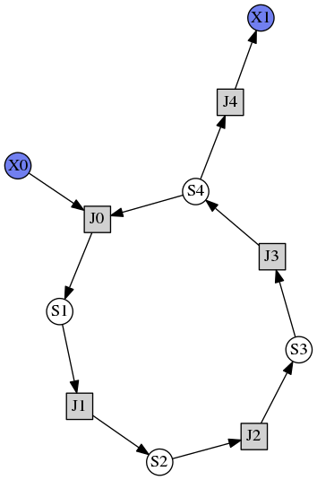
Draw diagram¶

This example shows how to draw a network diagram, requires graphviz.

import tellurium as te
te.setDefaultPlottingEngine('matplotlib')

r = te.loada('''
model feedback()
   // Reactions:http://localhost:8888/notebooks/core/tellurium_export.ipynb#
   J0: $X0 -> S1; (VM1 * (X0 - S1/Keq1))/(1 + X0 + S1 +   S4^h);
   J1: S1 -> S2; (10 * S1 - 2 * S2) / (1 + S1 + S2);
   J2: S2 -> S3; (10 * S2 - 2 * S3) / (1 + S2 + S3);
   J3: S3 -> S4; (10 * S3 - 2 * S4) / (1 + S3 + S4);
   J4: S4 -> $X1; (V4 * S4) / (KS4 + S4);

  // Species initializations:
  S1 = 0; S2 = 0; S3 = 0;
  S4 = 0; X0 = 10; X1 = 0;

  // Variable initialization:
  VM1 = 10; Keq1 = 10; h = 10; V4 = 2.5; KS4 = 0.5;
end''')

# simulate using variable step size
r.integrator.setValue('variable_step_size', True)
s = r.simulate(0, 50)
# draw the diagram
r.draw(width=200)
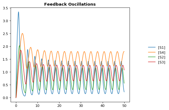
# and the plot
r.plot(s, title="Feedback Oscillations", ylabel="concentration", alpha=0.9);

Plotting multiple simulations¶

All plotting is done via the r.plot or te.plotArray functions. To plot multiple curves in one figure use the show=False setting.

import tellurium as te
te.setDefaultPlottingEngine('matplotlib')
import numpy as np
import matplotlib.pylab as plt

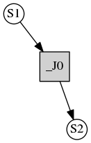
# Load a model and carry out a simulation generating 100 points
r = te.loada ('S1 -> S2; k1*S1; k1 = 0.1; S1 = 10')
r.draw(width=100)

# get colormap
# Colormap instances are used to convert data values (floats) from the interval [0, 1]
cmap = plt.get_cmap('Blues')

k1_values = np.linspace(start=0.1, stop=1.5, num=15)
max_k1 = max(k1_values)
for k, value in enumerate(k1_values):
    r.reset()
    r.k1 = value
    s = r.simulate(0, 30, 100)

    color = cmap((value+max_k1)/(2*max_k1))
    # use show=False to plot multiple curves in the same figure
    r.plot(s, show=False, title="Parameter variation k1", xtitle="time", ytitle="concentration",
          xlim=[-1, 31], ylim=[-0.1, 11])

te.show()

print('Reference Simulation: k1 = {}'.format(r.k1))
print('Parameter variation: k1 = {}'.format(k1_values))

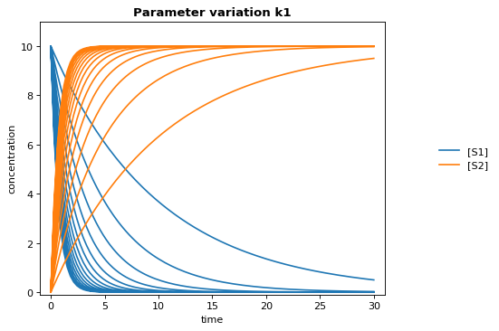
Reference Simulation: k1 = 1.5
Parameter variation: k1 = [ 0.1  0.2  0.3  0.4  0.5  0.6  0.7  0.8  0.9  1.   1.1  1.2  1.3  1.4  1.5]

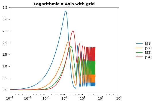
Logarithmic axis¶

The axis scale can be adapted with the xscale and yscale settings.

import tellurium as te
te.setDefaultPlottingEngine('matplotlib')
r = te.loadTestModel('feedback.xml')
r.integrator.variable_step_size = True
s = r.simulate(0, 50)
r.plot(s, logx=True, xlim=[10E-4, 10E2],
      title="Logarithmic x-Axis with grid", ylabel="concentration");

Model Reset¶

Use these routines reset your model back to particular states

class tellurium.tellurium.ExtendedRoadRunner(*args, **kwargs)[source]

resetAll()[source]¶

Reset all model variables to CURRENT init(X) values.

This resets all variables, S1, S2 etc to the CURRENT init(X) values. It also resets all parameters back to the values they had when the model was first loaded.

resetToOrigin()[source]¶

Reset model to state when first loaded.

This resets the model back to the state when it was FIRST loaded, this includes all init() and parameters such as k1 etc.

identical to:: r.reset(roadrunner.SelectionRecord.ALL)

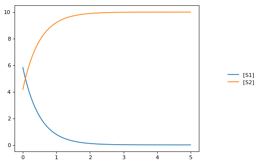
Reset model values¶

The reset function of a RoadRunner instance reset the system variables (usu. species concentrations) to their respective initial values. resetAll also resets parameters. resetToOrigin completely resets the model.

import tellurium as te
te.setDefaultPlottingEngine('matplotlib')

r = te.loada ('S1 -> S2; k1*S1; k1 = 0.1; S1 = 10')
r.integrator.setValue('variable_step_size', True)
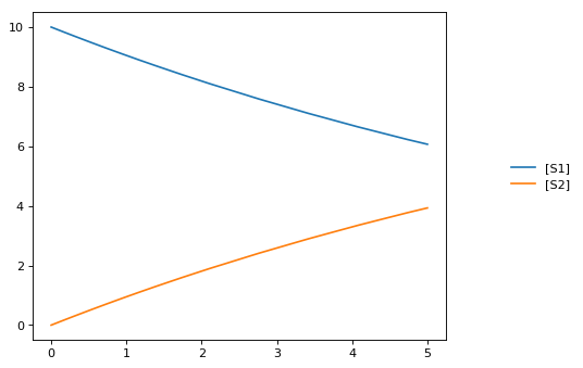
# simulate model
sim1 = r.simulate(0, 5)
print('*** sim1 ***')
r.plot(sim1)

# continue from end concentration of sim1
r.k1 = 2.0
sim2 = r.simulate(0, 5)
print('-- sim2 --')
print('continue simulation from final concentrations with changed parameter')
r.plot(sim2)

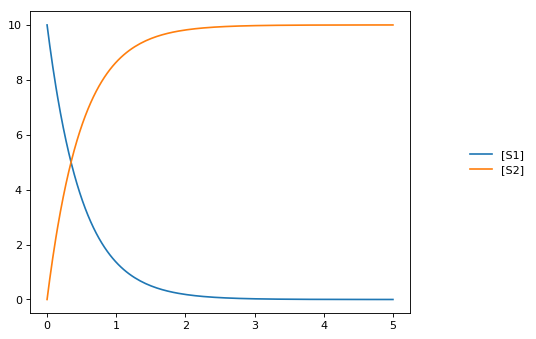
# Reset initial concentrations, does not affect the changed parameter
r.reset()
sim3 = r.simulate(0, 5)
print('-- sim3 --')
print('reset initial concentrations but keep changed parameter')
r.plot(sim3)

# Reset model to the state it was loaded
r.resetToOrigin()
sim4 = r.simulate(0, 5)
print('-- sim4 --')
print('reset all to origin')
r.plot(sim4);

* sim1 *

-- sim2 --
continue simulation from final concentrations with changed parameter

-- sim3 --
reset initial concentrations but keep changed parameter

-- sim4 --
reset all to origin

jarnac Short-cuts¶

Routines to support the Jarnac compatibility layer

class tellurium.tellurium.ExtendedRoadRunner(*args, **kwargs)[source]

bs()[source]¶

ExecutableModel.getBoundarySpeciesIds()

Returns a vector of boundary species Ids.

Parameters:	index (numpy.ndarray) – (optional) an index array indicating which items to return.
Returns:	a list of boundary species ids.

dv()[source]¶

ExecutableModel.getStateVector([stateVector])

Returns a vector of all the variables that represent the state of the system. The state is considered all values which change with the dynamics of the model. This would include all species which are produced or consumed by reactions, and all variables which are defined by rate rules.

Variables such as global parameters, compartments, or boundary species which do not change with the model dynamics are considered parameters and are thus not part of the state.

In performance critical applications, the optional stateVector array should be provided where the output variables will be written to.

Parameters:

stateVector (numpy.ndarray) –

an optional numpy array where the state vector variables will be written. If no state vector array is given, a new one will be constructed and returned.

This should be the same length as the model state vector.

Return type: numpy.ndarray

fjac()[source]¶

RoadRunner.getFullJacobian()

Compute the full Jacobian at the current operating point.

This is the Jacobian of ONLY the floating species.

fs()[source]¶

ExecutableModel.getFloatingSpeciesIds()

Return a list of floating species sbml ids.

rs()[source]¶

ExecutableModel.getReactionIds()

Returns a vector of reaction Ids.

Parameters:	index (numpy.ndarray) – (optional) an index array indicating which items to return.
Returns:	a list of reaction ids.

rv()[source]¶

ExecutableModel.getReactionRates([index])

Returns a vector of reaction rates (reaction velocity) for the current state of the model. The order of reaction rates is given by the order of Ids returned by getReactionIds()

Parameters:	index (numpy.ndarray) – (optional) an index array indicating which items to return.
Returns:	an array of reaction rates.
Return type:	numpy.ndarray

sm()[source]¶

RoadRunner.getFullStoichiometryMatrix()

Get the stoichiometry matrix that coresponds to the full model, even it it was converted via conservation conversion.

sv()[source]¶

ExecutableModel.getFloatingSpeciesConcentrations([index])

Returns a vector of floating species concentrations. The order of species is given by the order of Ids returned by getFloatingSpeciesIds()

Parameters:	index (numpy.ndarray) – (optional) an index array indicating which items to return.
Returns:	an array of floating species concentrations.
Return type:	numpy.ndarray

RoadRunner stores all initial conditions separately from the model state variables. This means that you can update the initial conditions at any time, and it does not affect the current state of the model. To reset the model, that is, reset it to its original state, or a new original state where what has changed the initial conditions use the reset() method.

The following methods allow access to the floating species initial condition values:

vs()[source]¶

ExecutableModel.getCompartmentIds([index])

Returns a vector of compartment identifier symbols.

Parameters:	index (None or numpy.ndarray) – A array of compartment indices indicating which compartment ids to return.
Returns:	a list of compartment ids.

Test Models¶

RoadRunner has built into it a number of predefined models that can be use to easily try and test tellurium.

tellurium.loadTestModel(string)[source]¶

Loads particular test model into roadrunner.

rr = te.loadTestModel('feedback.xml')

Returns:	RoadRunner instance with test model loaded

tellurium.getTestModel(string)[source]¶

SBML of given test model as a string.

# load test model as SBML
sbml = te.getTestModel('feedback.xml')
r = te.loadSBMLModel(sbml)
# simulate
r.simulate(0, 100, 20)

Returns:	SBML string of test model

tellurium.listTestModels()[source]¶

List roadrunner SBML test models.

print(te.listTestModels())

Returns:	list of test model paths

import tellurium as te

# To get the builtin models use listTestModels
print(te.listTestModels())

['EcoliCore.xml', 'test_1.xml', 'feedback.xml', 'linearPathwayClosed.xml', 'linearPathwayOpen.xml']

Load test model¶

# To load one of the test models use loadTestModel:
# r = te.loadTestModel('feedback.xml')
# result = r.simulate (0, 10, 100)
# r.plot (result)

# If you need to obtain the SBML for the test model, use getTestModel
sbml = te.getTestModel('feedback.xml')

# To look at one of the test model in Antimony form:
ant = te.sbmlToAntimony(te.getTestModel('feedback.xml'))
print(ant)

// Created by libAntimony v2.9.0
model *feedback()

  // Compartments and Species:
  compartment compartment_;
  species S1 in compartment_, S2 in compartment_, S3 in compartment_, S4 in compartment_;
  species $X0 in compartment_, $X1 in compartment_;

  // Reactions:
  J0: $X0 => S1; J0_VM1*(X0 - S1/J0_Keq1)/(1 + X0 + S1 + S4^J0_h);
  J1: S1 => S2; (10*S1 - 2*S2)/(1 + S1 + S2);
  J2: S2 => S3; (10*S2 - 2*S3)/(1 + S2 + S3);
  J3: S3 => S4; (10*S3 - 2*S4)/(1 + S3 + S4);
  J4: S4 => $X1; J4_V4*S4/(J4_KS4 + S4);

  // Species initializations:
  S1 = 0;
  S2 = 0;
  S3 = 0;
  S4 = 0;
  X0 = 10;
  X1 = 0;

  // Compartment initializations:
  compartment_ = 1;

  // Variable initializations:
  J0_VM1 = 10;
  J0_Keq1 = 10;
  J0_h = 10;
  J4_V4 = 2.5;
  J4_KS4 = 0.5;

  // Other declarations:
  const compartment_, J0_VM1, J0_Keq1, J0_h, J4_V4, J4_KS4;
end

Model Methods¶

Routines flattened from model, aves typing and easier for finding the methods

class tellurium.tellurium.ExtendedRoadRunner(*args, **kwargs)[source]

getBoundarySpeciesConcentrations([index])¶

Returns a vector of boundary species concentrations. The order of species is given by the order of Ids returned by getBoundarySpeciesIds()

Parameters:	index (numpy.ndarray) – (optional) an index array indicating which items to return.
Returns:	an array of the boundary species concentrations.
Return type:	numpy.ndarray.

given by the order of Ids returned by getBoundarySpeciesIds()

Parameters:	index (numpy.ndarray) – (optional) an index array indicating which items to return.
Returns:	an array of the boundary species concentrations.
Return type:	numpy.ndarray.

getBoundarySpeciesIds()¶

Returns a vector of boundary species Ids.

Parameters:	index (numpy.ndarray) – (optional) an index array indicating which items to return.
Returns:	a list of boundary species ids.

getCompartmentIds([index])¶

Returns a vector of compartment identifier symbols.

Parameters:	index (None or numpy.ndarray) – A array of compartment indices indicating which compartment ids to return.
Returns:	a list of compartment ids.

getCompartmentVolumes([index])¶

Returns a vector of compartment volumes. The order of volumes is given by the order of Ids returned by getCompartmentIds()

Parameters:	index (numpy.ndarray) – (optional) an index array indicating which items to return.
Returns:	an array of compartment volumes.
Return type:	numpy.ndarray.

getConservedMoietyValues([index])¶

Returns a vector of conserved moiety volumes. The order of values is given by the order of Ids returned by getConservedMoietyIds()

Parameters:	index (numpy.ndarray) – (optional) an index array indicating which items to return.
Returns:	an array of conserved moiety values.
Return type:	numpy.ndarray.

getFloatingSpeciesConcentrations([index])¶

Returns a vector of floating species concentrations. The order of species is given by the order of Ids returned by getFloatingSpeciesIds()

Parameters:	index (numpy.ndarray) – (optional) an index array indicating which items to return.
Returns:	an array of floating species concentrations.
Return type:	numpy.ndarray

RoadRunner stores all initial conditions separately from the model state variables. This means that you can update the initial conditions at any time, and it does not affect the current state of the model. To reset the model, that is, reset it to its original state, or a new original state where what has changed the initial conditions use the reset() method.

The following methods allow access to the floating species initial condition values:

getFloatingSpeciesIds()¶: Return a list of floating species sbml ids.

getGlobalParameterValues([index])¶

Return a vector of global parameter values. The order of species is given by the order of Ids returned by getGlobalParameterIds()

Parameters:	index (numpy.ndarray) – (optional) an index array indicating which items to return.
Returns:	an array of global parameter values.
Return type:	numpy.ndarray.

getNumBoundarySpecies()¶: Returns the number of boundary species in the model.

getNumCompartments()¶

Returns the number of compartments in the model.

Return type:	int

getNumConservedMoieties()¶

Returns the number of conserved moieties in the model.

Return type:	int

getNumFloatingSpecies()¶: Returns the number of floating species in the model.

getNumGlobalParameters()¶: Returns the number of global parameters in the model.

getNumReactions()¶: Returns the number of reactions in the model.

getRatesOfChange()[source]¶

Rate of change of all state variables in the model.

Returns:	rate of change of all state variables (eg species) in the model.

getReactionIds()¶

Returns a vector of reaction Ids.

Parameters:	index (numpy.ndarray) – (optional) an index array indicating which items to return.
Returns:	a list of reaction ids.

getReactionRates([index])¶

Returns a vector of reaction rates (reaction velocity) for the current state of the model. The order of reaction rates is given by the order of Ids returned by getReactionIds()

Parameters:	index (numpy.ndarray) – (optional) an index array indicating which items to return.
Returns:	an array of reaction rates.
Return type:	numpy.ndarray